The prime number theorem

Compares the prime-counting function \(\pi(x)\) with Gauss’s logarithmic integral \(\operatorname{li}(x)\) and Legendre-style \(x/\ln x\) up to ten million. Both ratios tend to 1, as Hadamard and de la Vallée Poussin proved in 1896, but \(\operatorname{li}(x)\) is far more accurate.

import matplotlib.pyplot as plt
import numpy as np

from mathematicskit.number_theory import logarithmic_integral, prime_counting

pi(x) against its two approximations

xs = np.unique(np.logspace(2, 7, 60).astype(np.int64))
pi_x = prime_counting(xs)
li_x = logarithmic_integral(xs.astype(float))
x_log_x = xs / np.log(xs)
for x in (10**3, 10**5, 10**7):
    i = np.searchsorted(xs, x)
    print(f"x = {xs[i]:>9}: pi(x) = {pi_x[i]:>7}, li(x) = {li_x[i]:>10.1f}, x/ln x = {x_log_x[i]:>10.1f}")

fig, ax = plt.subplots()
ax.semilogx(xs, li_x / pi_x, label="li(x) / pi(x)")
ax.semilogx(xs, x_log_x / pi_x, label="(x / ln x) / pi(x)")
ax.axhline(1.0, color="0.5", ls=":")
ax.set_xlabel("x")
ax.set_ylabel("ratio")
ax.set_title("Both approximations are asymptotic to pi(x)")
ax.legend()
plt.show()

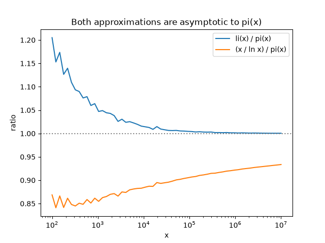
x =      1039: pi(x) =     175, li(x) =      183.2, x/ln x =      149.6
x =    112421: pi(x) =   10659, li(x) =    10703.1, x/ln x =     9666.5
x =  10000000: pi(x) =  664579, li(x) =   664918.4, x/ln x =   620420.7