Lorenz’s butterfly effect: deterministic chaos

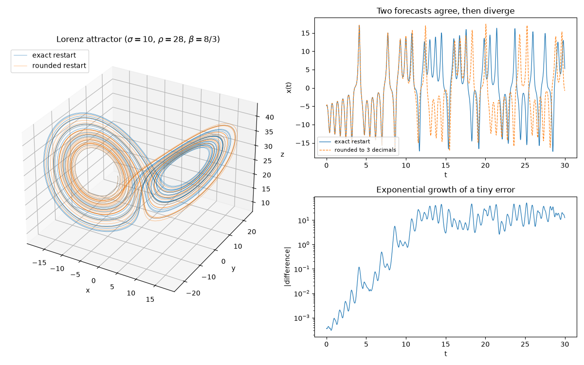
Lorenz’s 1963 convection model \(\dot x = \sigma(y - x)\), \(\dot y = x(\rho - z) - y\), \(\dot z = xy - \beta z\) is fully deterministic, yet for \(\sigma = 10\), \(\rho = 28\), \(\beta = 8/3\) its orbits wind forever around a butterfly-shaped strange attractor. This script repeats Lorenz’s accidental experiment: restart a run from a state rounded to three decimal places, and watch the two forecasts agree for a while, then diverge completely.

import matplotlib.pyplot as plt
import numpy as np

from mathematicskit.ode_dynamics.systems.chaotic_flows import LorenzSystem, lorenz_fixed_points
from mathematicskit.ode_dynamics.systems.stability import numerical_jacobian

Every fixed point is unstable

Linearizing at the origin and at the two convection-roll states \(C_\pm\) shows each has an eigenvalue with positive real part, so no orbit can settle down – yet the flow stays bounded.

system = LorenzSystem([1.0, 1.0, 1.0])
for fp in lorenz_fixed_points():
    eig = np.linalg.eigvals(numerical_jacobian(system.rhs, fp))
    print(f"fixed point {np.round(fp, 3)}: max Re(eigenvalue) = {eig.real.max():+.3f}")

fixed point [0. 0. 0.]: max Re(eigenvalue) = +11.828
fixed point [ 8.485  8.485 27.   ]: max Re(eigenvalue) = +0.094
fixed point [-8.485 -8.485 27.   ]: max Re(eigenvalue) = +0.094

Lorenz’s rounding experiment

Run to \(t = 10\), then restart once from the exact state and once from the state rounded to three decimals, as Lorenz did from his printout.

burn_in = system.integrate((0.0, 10.0), dt=1e-3, method="rk4")
exact0 = burn_in.y[-1]
rounded0 = np.round(exact0, 3)
print(f"initial difference after rounding: {np.linalg.norm(exact0 - rounded0):.2e}")

t_span = (0.0, 30.0)
exact = LorenzSystem(exact0).integrate(t_span, dt=1e-3, method="rk4")
rounded = LorenzSystem(rounded0).integrate(t_span, dt=1e-3, method="rk4")
separation = np.linalg.norm(exact.y - rounded.y, axis=1)
print(f"separation at t = 30: {separation[-1]:.2f} (attractor width ~ 40)")

# Slope of log(separation) over the exponential-growth phase approximates
# the largest Lyapunov exponent (roughly; about 0.91 for these parameters).
growth = (separation > 1e-3) & (separation < 1.0)
slope = np.polyfit(exact.t[growth], np.log(separation[growth]), 1)[0]
print(f"estimated largest Lyapunov exponent: {slope:.2f} (accepted value ~0.91)")

initial difference after rounding: 3.66e-04
separation at t = 30: 12.49 (attractor width ~ 40)
estimated largest Lyapunov exponent: 0.76 (accepted value ~0.91)

The butterfly and the diverging forecasts

fig = plt.figure(figsize=(12, 7.5))
ax3d = fig.add_subplot(2, 2, (1, 3), projection="3d")
ax3d.plot(*exact.y.T, lw=0.4, color="tab:blue", label="exact restart")
ax3d.plot(*rounded.y.T, lw=0.4, color="tab:orange", alpha=0.8, label="rounded restart")
ax3d.set_xlabel("x")
ax3d.set_ylabel("y")
ax3d.set_zlabel("z")
ax3d.set_title(r"Lorenz attractor ($\sigma=10$, $\rho=28$, $\beta=8/3$)")
ax3d.legend(loc="upper left")

ax = fig.add_subplot(2, 2, 2)
ax.plot(exact.t, exact.y[:, 0], lw=0.9, label="exact restart")
ax.plot(rounded.t, rounded.y[:, 0], lw=0.9, ls="--", label="rounded to 3 decimals")
ax.set_xlabel("t")
ax.set_ylabel("x(t)")
ax.set_title("Two forecasts agree, then diverge")
ax.legend(loc="lower left", fontsize=8)

ax = fig.add_subplot(2, 2, 4)
ax.semilogy(exact.t, separation, lw=0.9)
ax.set_xlabel("t")
ax.set_ylabel("|difference|")
ax.set_title("Exponential growth of a tiny error")
fig.tight_layout()

plt.show()