The Rossler attractor

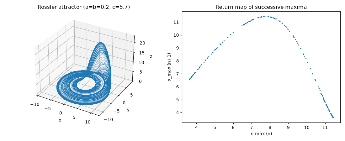
Rossler’s flow has a single nonlinear term, yet for \(a = b = 0.2\), \(c = 5.7\) it settles onto a chaotic attractor: orbits spiral outward near the plane \(z \approx 0\), are lifted and folded back when \(x\) exceeds \(c\), and never exactly repeat. Plotting each loop’s maximum of \(x\) against the previous one gives a Lorenz-style return map, a thin single-humped curve.

import matplotlib.pyplot as plt
import numpy as np

from mathematicskit.ode_dynamics.systems.chaotic_flows import RosslerSystem, rossler_fixed_points

print("fixed points:\n", np.round(rossler_fixed_points(), 4))

system = RosslerSystem([1.0, 1.0, 0.0])
system.integrate((0.0, 100.0), dt=1e-2, method="rk4")
traj = system.integrate((100.0, 1100.0), dt=1e-2, method="rk4")
x, y, z = traj.y.T

fixed points:
 [[ 7.00000e-03 -3.51000e-02  3.51000e-02]
 [ 5.69300e+00 -2.84649e+01  2.84649e+01]]

The attractor and its return map

peaks = x[1:-1][(x[1:-1] > x[:-2]) & (x[1:-1] > x[2:])]
fig = plt.figure(figsize=(11, 4.5))
ax3d = fig.add_subplot(1, 2, 1, projection="3d")
ax3d.plot(x, y, z, lw=0.3)
ax3d.set_xlabel("x")
ax3d.set_ylabel("y")
ax3d.set_zlabel("z")
ax3d.set_title("Rossler attractor (a=b=0.2, c=5.7)")
ax = fig.add_subplot(1, 2, 2)
ax.plot(peaks[:-1], peaks[1:], ".", ms=3)
ax.set_xlabel("x_max (n)")
ax.set_ylabel("x_max (n+1)")
ax.set_title("Return map of successive maxima")
fig.tight_layout()

plt.show()