Poincaré’s classification of fixed points: nodes, saddles, spirals, centers

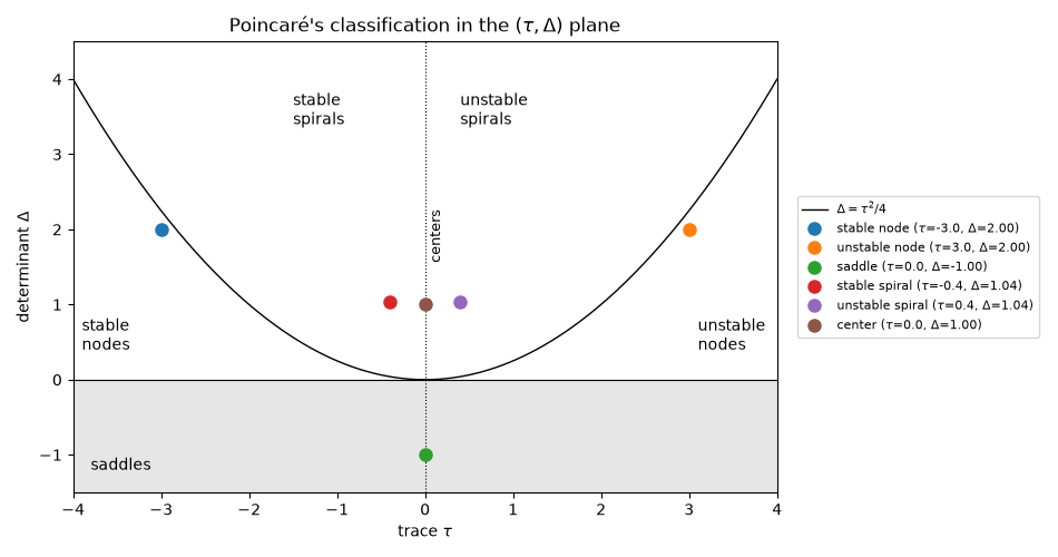
Poincaré’s qualitative theory sorts a planar fixed point into one of four types – node, saddle, spiral (focus), or center – using only the eigenvalues of the linearized flow, without solving the equations. The eigenvalues depend only on the Jacobian’s trace \(\tau\) and determinant \(\Delta\), so every type occupies its own region of the \((\tau, \Delta)\) plane. This script classifies six canonical matrices, draws their phase portraits, and places each one on Poincaré’s trace-determinant diagram.

import matplotlib.pyplot as plt
import numpy as np

from mathematicskit.ode_dynamics.systems.phase_portrait import Linear2D
from mathematicskit.ode_dynamics.systems.stability import classify_fixed_point_2d

Poincaré’s four types in six canonical linear systems

matrices = {
    "stable node": np.array([[-1.0, 0.0], [0.0, -2.0]]),
    "unstable node": np.array([[1.0, 0.0], [0.0, 2.0]]),
    "saddle": np.array([[1.0, 0.0], [0.0, -1.0]]),
    "stable spiral": np.array([[-0.2, 1.0], [-1.0, -0.2]]),
    "unstable spiral": np.array([[0.2, 1.0], [-1.0, 0.2]]),
    "center": np.array([[0.0, 1.0], [-1.0, 0.0]]),
}

fig, axes = plt.subplots(2, 3, figsize=(11, 7))
rng = np.random.default_rng(0)
for ax, (name, A) in zip(axes.ravel(), matrices.items()):
    result = classify_fixed_point_2d(A)
    print(f"{name:>16s}: eigenvalues={np.round(result.eigenvalues, 3)}, classified as '{result.classification}'")
    for _ in range(6):
        state0 = rng.uniform(-1, 1, 2)
        system = Linear2D(state0, A=A)
        traj = system.integrate((0.0, 8.0), dt=1e-3, method="rk4")
        ax.plot(traj.y[:, 0], traj.y[:, 1], lw=0.8)
    ax.plot(0, 0, "ko", ms=4)
    ax.set_title(name)
    ax.set_xlim(-2, 2)
    ax.set_ylim(-2, 2)
fig.suptitle("Poincaré's fixed-point types (phase portraits)")
fig.tight_layout()

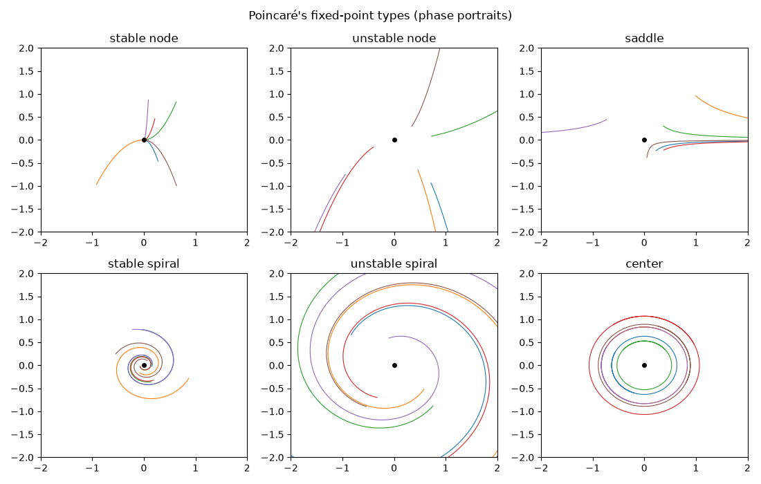
    stable node: eigenvalues=[-1.+0.j -2.+0.j], classified as 'stable node'
  unstable node: eigenvalues=[2.+0.j 1.+0.j], classified as 'unstable node'
         saddle: eigenvalues=[ 1.+0.j -1.+0.j], classified as 'saddle'
  stable spiral: eigenvalues=[-0.2+1.j -0.2-1.j], classified as 'stable spiral'
unstable spiral: eigenvalues=[0.2+1.j 0.2-1.j], classified as 'unstable spiral'
         center: eigenvalues=[0.+1.j 0.-1.j], classified as 'center'

The trace-determinant diagram

The parabola \(\Delta = \tau^2/4\) separates nodes (real eigenvalues) from spirals (complex eigenvalues); \(\Delta < 0\) is always a saddle, and the positive \(\Delta\) axis (\(\tau = 0\)) holds the centers.

fig, ax = plt.subplots(figsize=(9.5, 5))
tau = np.linspace(-4.0, 4.0, 400)
ax.plot(tau, tau**2 / 4, "k-", lw=1, label=r"$\Delta = \tau^2/4$")
ax.axhline(0, color="k", lw=0.8)
ax.axvline(0, color="k", lw=0.8, ls=":")
ax.fill_between(tau, -1.5, 0, color="0.9")
for name, A in matrices.items():
    t, d = np.trace(A), np.linalg.det(A)
    ax.plot(t, d, "o", ms=8, label=f"{name} ($\\tau$={t:.1f}, $\\Delta$={d:.2f})")
ax.text(-3.8, -1.2, "saddles", fontsize=10)
ax.text(-3.9, 0.4, "stable\nnodes", fontsize=10)
ax.text(3.1, 0.4, "unstable\nnodes", fontsize=10)
ax.text(-1.5, 3.4, "stable\nspirals", fontsize=10)
ax.text(0.4, 3.4, "unstable\nspirals", fontsize=10)
ax.text(0.05, 1.6, "centers", fontsize=9, rotation=90)
ax.set_xlim(-4.0, 4.0)
ax.set_ylim(-1.5, 4.5)
ax.set_xlabel(r"trace $\tau$")
ax.set_ylabel(r"determinant $\Delta$")
ax.set_title("Poincaré's classification in the $(\\tau, \\Delta)$ plane")
ax.legend(fontsize=8, loc="center left", bbox_to_anchor=(1.02, 0.5))
fig.tight_layout()

plt.show()