Karmarkar’s interior-point method: the central path

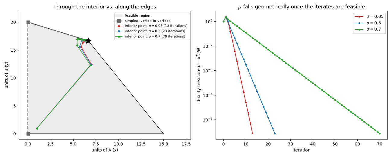
The simplex method walks the edges of the feasible polygon. Karmarkar (1984) cut through its interior instead, with an algorithm that was both polynomial-time and fast in practice. Its descendants, the primal-dual path-following methods used by every modern LP solver, track the central path: the points where every product \(x_i s_i\) of a primal variable and its dual slack equals the same \(\mu\). As \(\mu \to 0\) the path ends at the optimal vertex.

The problem is the production LP of the simplex example: maximize \(3x + 5y\) subject to \(x + 2y \leq 40\), \(2x + y \leq 30\).

import matplotlib.pyplot as plt
import numpy as np

from mathematicskit.optimization import interior_point_lp, linear_program

c = np.array([-3.0, -5.0])  # minimize the negated profit
a_ub = np.array([[1.0, 2.0], [2.0, 1.0]])
b_ub = np.array([40.0, 30.0])

Interior-point iterates

result = interior_point_lp(c, a_ub, b_ub, sigma=0.3, eta=0.9)
for k, (x, mu) in enumerate(zip(result.path, result.extra["duality_measure"], strict=False)):
    if k < 6 or k == len(result.path) - 1:
        print(f"iterate {k:2d}: (x, y) = ({x[0]:7.3f}, {x[1]:7.3f}), profit {-c @ x:8.3f}, mu = {mu:.1e}")
print(f"converged in {result.iterations} iterations to {result.x.round(6)}")

for method in ("highs-ipm", "highs-ds"):
    check = linear_program(c, a_ub=a_ub, b_ub=b_ub, method=method)
    print(f"linprog {method:9s}: {check.x.round(6)}, profit {-check.fun:.6f}")

iterate  0: (x, y) = (  1.000,   1.000), profit    8.000, mu = 1.0e+00
iterate  1: (x, y) = (  6.976,  12.376), profit   82.808, mu = 2.2e+00
iterate  2: (x, y) = (  5.731,  15.640), profit   95.394, mu = 1.0e+00
iterate  3: (x, y) = (  5.980,  16.857), profit  102.227, mu = 3.1e-01
iterate  4: (x, y) = (  6.389,  16.772), profit  103.028, mu = 1.2e-01
iterate  5: (x, y) = (  6.577,  16.702), profit  103.238, mu = 4.3e-02
iterate 23: (x, y) = (  6.667,  16.667), profit  103.333, mu = 7.3e-10
converged in 23 iterations to [ 6.666667 16.666667]
linprog highs-ipm: [ 6.666667 16.666667], profit 103.333333
linprog highs-ds : [ 6.666667 16.666667], profit 103.333333

Centring: how close the iterates stay to the central path

A small centring parameter \(\sigma\) aims straight at the optimum and hugs the boundary; a larger one follows the central path through the middle of the polygon, at the cost of more iterations. The simplex path from the earlier example, \((0,0) \to (0,20) \to (20/3, 50/3)\), runs along the edges.

polygon = np.array([[0.0, 0.0], [15.0, 0.0], [20.0 / 3.0, 50.0 / 3.0], [0.0, 20.0]])
simplex_path = np.array([[0.0, 0.0], [0.0, 20.0], [20.0 / 3.0, 50.0 / 3.0]])

fig, (ax0, ax1) = plt.subplots(1, 2, figsize=(13, 5.2))
ax0.fill(*polygon.T, color="0.92", label="feasible region")
ax0.plot(*np.vstack([polygon, polygon[:1]]).T, "k-", lw=1)
ax0.plot(*simplex_path.T, "s--", color="0.4", ms=7, lw=2, label="simplex (vertex to vertex)")
for sigma, color in [(0.05, "tab:red"), (0.3, "tab:blue"), (0.7, "tab:green")]:
    run = interior_point_lp(c, a_ub, b_ub, sigma=sigma, eta=0.9)
    ax0.plot(*run.path.T, "o-", color=color, ms=4, lw=1.2, label=rf"interior point, $\sigma = {sigma}$ ({run.iterations} iterations)")
    ax1.semilogy(run.extra["duality_measure"], "o-", color=color, ms=3, label=rf"$\sigma = {sigma}$")
ax0.plot(20 / 3, 50 / 3, "k*", ms=16)
ax0.set_xlim(-1, 18)
ax0.set_ylim(-1, 22)
ax0.set_xlabel("units of A (x)")
ax0.set_ylabel("units of B (y)")
ax0.set_title("Through the interior vs. along the edges")
ax0.legend(fontsize=8, loc="upper right")

ax1.set_xlabel("iteration")
ax1.set_ylabel(r"duality measure $\mu = x^T s / N$")
ax1.set_title(r"$\mu$ falls geometrically once the iterates are feasible")
ax1.legend()
fig.tight_layout()

plt.show()