Branch and bound: integer versus relaxed optimum

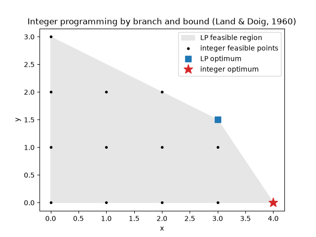
The LP relaxation of an integer program can have a fractional optimum that rounding does not repair. Branch and bound (Land and Doig, 1960) finds the true integer optimum; here it is at a different vertex from the relaxation’s.

import matplotlib.pyplot as plt
import numpy as np

from mathematicskit.optimization import integer_linear_program, linear_program

maximize 5x + 4y s.t. 6x + 4y <= 24, x + 2y <= 6

c = np.array([-5.0, -4.0])
a_ub = np.array([[6.0, 4.0], [1.0, 2.0]])
b_ub = np.array([24.0, 6.0])
relaxed = linear_program(c, a_ub=a_ub, b_ub=b_ub)
integer = integer_linear_program(c, a_ub=a_ub, b_ub=b_ub)
print(f"LP relaxation: x = {relaxed.x}, objective {-relaxed.fun:.2f}")
print(f"integer optimum: x = {integer.x.round() + 0.0}, objective {-integer.fun:.2f}")
print(f"rounding the relaxation down gives {np.floor(relaxed.x)}, objective {5 * np.floor(relaxed.x[0]) + 4 * np.floor(relaxed.x[1]):.2f}")

LP relaxation: x = [3.  1.5], objective 21.00
integer optimum: x = [4. 0.], objective 20.00
rounding the relaxation down gives [3. 1.], objective 19.00

Feasible region and lattice points

fig, ax = plt.subplots()
ax.fill([0, 4, 3, 0], [0, 0, 1.5, 3], color="0.9", label="LP feasible region")
gx, gy = np.meshgrid(np.arange(5), np.arange(4))
feasible = (6 * gx + 4 * gy <= 24) & (gx + 2 * gy <= 6)
ax.plot(gx[feasible], gy[feasible], "k.", label="integer feasible points")
ax.plot(*relaxed.x, "s", color="tab:blue", ms=9, label="LP optimum")
ax.plot(*integer.x, "*", color="tab:red", ms=14, label="integer optimum")
ax.set_xlabel("x")
ax.set_ylabel("y")
ax.legend()
ax.set_title("Integer programming by branch and bound (Land & Doig, 1960)")

Text(0.5, 1.0, 'Integer programming by branch and bound (Land & Doig, 1960)')