Finite elements: Galerkin’s hat functions on an uneven mesh

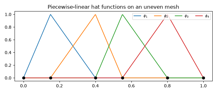
Richard Courant (1943) proposed piecewise-linear approximations on a triangulation, and aircraft engineers (Turner, Clough, Martin and Topp, 1956) turned the idea into the finite element method. Instead of differencing \(u'' = f\), ask the weak form \(-\int u'v' = \int f v\) to hold for every “hat” function \(v\) on the mesh. The mesh can be refined exactly where the solution needs it. This script shows the hat-function basis, solves a boundary layer on a graded mesh, and shows that 1D linear elements are exact at the nodes.

import matplotlib.pyplot as plt
import numpy as np

from mathematicskit.pde import fem_poisson_1d, solve_poisson_1d

The hat-function basis

nodes = np.array([0.0, 0.15, 0.4, 0.55, 0.8, 1.0])
x = np.linspace(0, 1, 500)
fig1, ax1 = plt.subplots(figsize=(7, 3))
for i in range(1, len(nodes) - 1):
    hat = np.interp(x, nodes, np.eye(len(nodes))[i])
    ax1.plot(x, hat, label=rf"$\phi_{i}$")
ax1.plot(nodes, 0 * nodes, "ko")
ax1.set_title("Piecewise-linear hat functions on an uneven mesh")
ax1.legend(fontsize=8, ncol=4)
fig1.tight_layout()

A boundary layer on a graded mesh

\(u'' = f\) with \(u = e^{-x/\epsilon}\)-like behavior near \(x = 0\): clustering 20 elements near the layer beats 20 uniform ones.

eps = 0.02
exact = lambda s: np.exp(-s / eps)
source = lambda s: np.exp(-s / eps) / eps**2
graded = np.linspace(0, 1, 21) ** 3
uniform = fem_poisson_1d(source, n_elements=20, ua=1.0, ub=exact(1.0), quad_points=6)
refined = fem_poisson_1d(source, nodes=graded, ua=1.0, ub=exact(1.0), quad_points=6)

fig2, ax2 = plt.subplots(figsize=(7, 4))
ax2.plot(x, exact(x), color="black", lw=2, label="exact")
ax2.plot(uniform.x, uniform.u, "o-", ms=4, label="20 uniform elements")
ax2.plot(refined.x, refined.u, "s-", ms=4, label="20 graded elements")
ax2.set_xlim(0, 0.3)
ax2.set_xlabel("$x$")
ax2.legend()
ax2.set_title("Refine the mesh where the solution varies")
fig2.tight_layout()
for name, s in (("uniform", uniform), ("graded", refined)):
    xs = np.linspace(0, 1, 2001)
    print(f"{name:>8} mesh: max error of the piecewise-linear solution = {np.max(np.abs(np.interp(xs, s.x, s.u) - exact(xs))):.3f}")

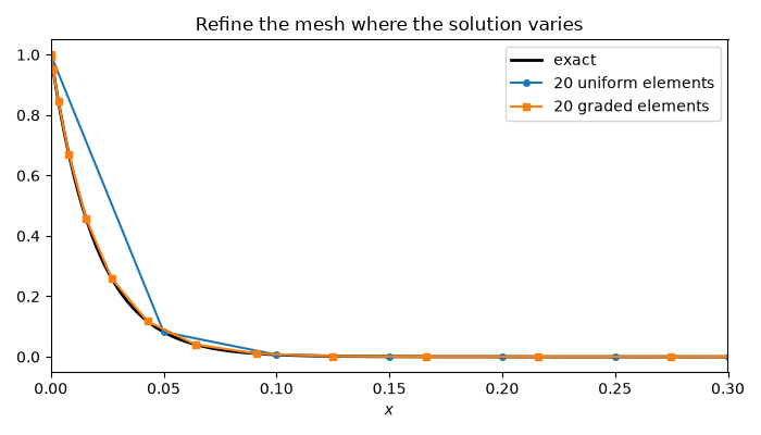
uniform mesh: max error of the piecewise-linear solution = 0.265
 graded mesh: max error of the piecewise-linear solution = 0.014

Exact at the nodes

In 1D, the Galerkin solution interpolates the true solution at the mesh nodes (up to quadrature error), even where finite differences on the same points are only second-order accurate.

f = lambda s: -(np.pi**2) * np.sin(np.pi * s)
fem = fem_poisson_1d(f, n_elements=8, quad_points=8)
fd = solve_poisson_1d(f, 0.0, 1.0, 9)
print(f"finite elements, max nodal error:   {np.max(np.abs(fem.u - np.sin(np.pi * fem.x))):.1e}")
print(f"finite differences, max nodal error: {np.max(np.abs(fd.u - np.sin(np.pi * fd.x))):.1e}")

plt.show()

finite elements, max nodal error:   1.2e-16
finite differences, max nodal error: 1.3e-02