De Moivre-Laplace and the central limit theorem: the bell curve emerges

De Moivre (1733) showed that the binomial distribution, suitably standardized, approaches the normal curve for large \(n\). Laplace (1810) extended this to sums of many independent variables of almost any distribution: the standardized mean \(Z = (\bar X_n - \mu)/(\sigma/\sqrt n)\) tends to \(\mathcal N(0, 1)\), whatever the shape of the summands.

import matplotlib.pyplot as plt
import numpy as np
from scipy import stats

from mathematicskit.probability import Binomial, Exponential, Normal
from mathematicskit.probability.systems.limit_theorems import central_limit_theorem_sample_means
from mathematicskit.probability.visualizers.plots import plot_clt_histogram

standard_normal = Normal(mu=0.0, sigma=1.0)

De Moivre: standardized binomial PMFs approach the normal density

p = 0.2
z_grid = np.linspace(-4.0, 4.0, 400)
fig, axes = plt.subplots(1, 3, figsize=(10, 3.2), sharey=True)
for ax, n in zip(axes, (5, 30, 300)):
    binomial = Binomial(n=n, p=p)
    ks = np.arange(n + 1)
    z = (ks - binomial.mean) / binomial.std
    # rescale the PMF by the lattice spacing 1/sigma so it compares with a density
    ax.bar(z, binomial.pmf(ks) * binomial.std, width=1.0 / binomial.std, alpha=0.6, label=f"Binomial({n}, {p})")
    ax.plot(z_grid, standard_normal.pdf(z_grid), "k", lw=1.5, label="N(0, 1)")
    ax.set_xlim(-4.0, 4.0)
    ax.set_title(f"n = {n}")
    ax.set_xlabel("standardized count")
axes[0].set_ylabel("density")
axes[0].legend(fontsize=7, loc="upper left")
fig.suptitle("De Moivre-Laplace theorem")
fig.tight_layout()

for n in (5, 30, 300, 3000):
    binomial = Binomial(n=n, p=p)
    ks = np.arange(n + 1)
    gap = np.max(np.abs(binomial.cdf(ks) - standard_normal.cdf((ks + 0.5 - binomial.mean) / binomial.std)))
    print(f"n={n:>5}: max CDF gap to the normal approximation = {gap:.4f}")

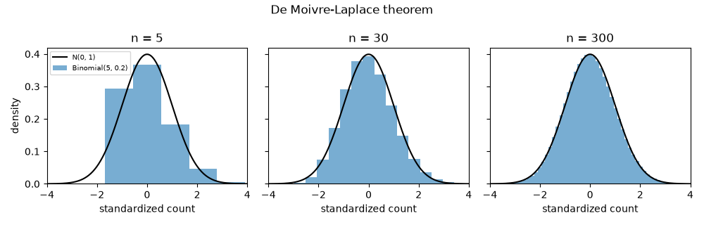
n=    5: max CDF gap to the normal approximation = 0.0396
n=   30: max CDF gap to the normal approximation = 0.0178
n=  300: max CDF gap to the normal approximation = 0.0057
n= 3000: max CDF gap to the normal approximation = 0.0018

Laplace: sample means of a skewed distribution become normal too

skewed = Exponential(rate=1.0)
z = central_limit_theorem_sample_means(skewed, n=200, n_trials=5000, seed=0)
_, p_value = stats.kstest(z, "norm")
print(f"Exponential(1) sample means, n=200: KS test against N(0, 1), p-value = {p_value:.4f}")
ax = plot_clt_histogram(z)
ax.set_title("Central limit theorem: standardized means of Exponential(1) samples")

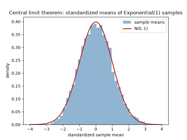
Exponential(1) sample means, n=200: KS test against N(0, 1), p-value = 0.7715

Text(0.5, 1.0, 'Central limit theorem: standardized means of Exponential(1) samples')