Brownian motion

Sample paths of standard Brownian motion spread like \(\sqrt{t}\): at time \(t\), \(W(t) \sim \mathcal N(0, t)\), so about 95% of paths lie within \(\pm 2\sqrt t\). The quadratic variation \(\sum (\Delta W)^2\) equals \(t\), the signature of a path that is continuous but nowhere differentiable.

import matplotlib.pyplot as plt
import numpy as np

from mathematicskit.probability import brownian_motion

Paths and the 2-sigma envelope

result = brownian_motion(n_paths=2000, n_steps=1000, t_max=1.0, seed=0)
t = result.times
fig, ax = plt.subplots()
ax.plot(t, result.paths[:30].T, lw=0.8)
ax.plot(t, 2 * np.sqrt(t), "k--", t, -2 * np.sqrt(t), "k--")
ax.set_xlabel("t")
ax.set_ylabel("W(t)")
ax.set_title(r"Brownian motion with $\pm 2\sqrt{t}$ envelope")

inside = np.mean(np.abs(result.paths[:, -1]) <= 2.0)
print(f"Var W(1) = {result.paths[:, -1].var():.4f} (theory 1)")
print(f"fraction within 2 sd at t = 1: {inside:.4f} (theory 0.9545)")

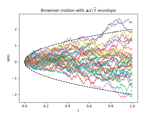
Var W(1) = 1.0174 (theory 1)
fraction within 2 sd at t = 1: 0.9560 (theory 0.9545)

Quadratic variation

fine = brownian_motion(n_paths=1, n_steps=100000, t_max=1.0, seed=1)
qv = np.cumsum(np.diff(fine.paths[0]) ** 2)
print(f"quadratic variation on [0, 1]: {qv[-1]:.4f} (theory 1)")

quadratic variation on [0, 1]: 0.9931 (theory 1)