Galton’s heights and Pearson’s correlation

Simulates parent and child heights in the spirit of Francis Galton’s 1880s data: the two are positively correlated, but tall parents have children who are on average less extreme – “regression toward the mean”. Pearson’s r measures the strength of that linear relation.

import matplotlib.pyplot as plt
import numpy as np

from mathematicskit.statistics import linear_regression, pearson_correlation

Parent and child heights

rng = np.random.default_rng(0)
parent = rng.normal(loc=68.0, scale=1.8, size=400)
child = 68.0 + 0.65 * (parent - 68.0) + rng.normal(scale=2.0, size=400)

result = pearson_correlation(parent, child)
print(f"Pearson r = {result.coefficient:.3f} (n={result.n}, p={result.p_value:.2e})")

Pearson r = 0.555 (n=400, p=1.06e-33)

The slope of the standardized fit is r itself

fit = linear_regression(parent, child)
slope = fit.coefficients[1]
print(f"regression slope = {slope:.3f}, r * s_child / s_parent = {result.coefficient * child.std() / parent.std():.3f}")

fig, ax = plt.subplots()
ax.scatter(parent, child, s=8, alpha=0.5)
grid = np.linspace(parent.min(), parent.max(), 50)
ax.plot(grid, fit.coefficients[0] + slope * grid, "C1", label=f"fit, slope {slope:.2f}")
ax.plot(grid, grid, "k--", lw=1, label="slope 1 (no regression to the mean)")
ax.set_xlabel("parent height (in)")
ax.set_ylabel("child height (in)")
ax.set_title(f"r = {result.coefficient:.2f}")
ax.legend()

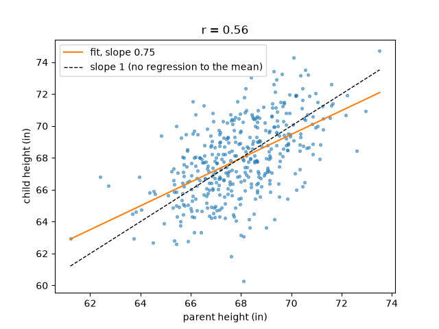
regression slope = 0.746, r * s_child / s_parent = 0.746

<matplotlib.legend.Legend object at 0x11ce34ec0>