Gauss’s normal law of errors

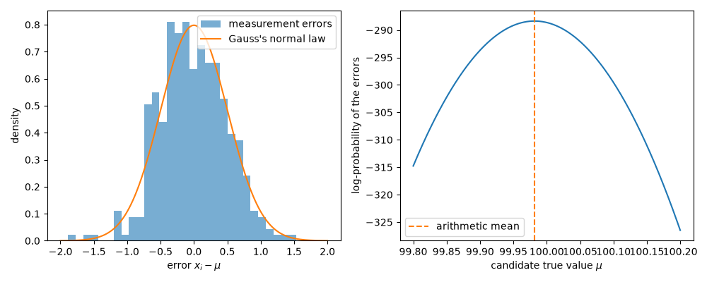
Repeated measurements of one quantity scatter around its true value. Gauss (1809) asked which error law makes the arithmetic mean of the measurements the most probable value of the quantity, and found the normal law. This example simulates noisy measurements, compares their errors with the normal curve, and checks that the mean both maximizes the normal error probability and minimizes the sum of squared errors.

import matplotlib.pyplot as plt
import numpy as np
from scipy import stats

from mathematicskit.statistics import descriptive_stats, maximum_likelihood_fit

Repeated measurements of a known length

rng = np.random.default_rng(0)
true_value = 100.0
sigma = 0.5
measurements = true_value + rng.normal(scale=sigma, size=400)
errors = measurements - true_value

summary = descriptive_stats(errors)
print(f"error mean = {summary.mean:+.4f}, error std = {summary.std:.4f} (sigma = {sigma})")
print(f"skewness = {summary.skewness:+.3f}, excess kurtosis = {summary.kurtosis:+.3f} (normal: 0, 0)")

error mean = -0.0183, error std = 0.4982 (sigma = 0.5)
skewness = -0.037, excess kurtosis = +0.310 (normal: 0, 0)

The mean is the most probable value

Under the normal error law, the probability of the observed errors for a candidate true value \(\mu\) is proportional to \(\exp(-\sum_i (x_i - \mu)^2 / 2\sigma^2)\), so maximizing it is the same as minimizing the sum of squared errors – least squares.

fit = maximum_likelihood_fit(measurements, "norm")
print(f"most probable value = {fit.params[0]:.4f}, arithmetic mean = {measurements.mean():.4f}")

candidates = np.linspace(99.8, 100.2, 401)
log_prob = np.array([np.sum(stats.norm.logpdf(measurements, loc=m, scale=sigma)) for m in candidates])
sse = np.array([np.sum((measurements - m) ** 2) for m in candidates])
print(f"argmax log-probability = {candidates[np.argmax(log_prob)]:.3f}, argmin squared error = {candidates[np.argmin(sse)]:.3f}")

most probable value = 99.9817, arithmetic mean = 99.9817
argmax log-probability = 99.982, argmin squared error = 99.982

Plot the error law and the most-probable-value curve

fig, (ax1, ax2) = plt.subplots(1, 2, figsize=(10, 4))
ax1.hist(errors, bins=30, density=True, alpha=0.6, label="measurement errors")
grid = np.linspace(-4 * sigma, 4 * sigma, 300)
ax1.plot(grid, stats.norm.pdf(grid, scale=sigma), "C1", label="Gauss's normal law")
ax1.set_xlabel("error $x_i - \\mu$")
ax1.set_ylabel("density")
ax1.legend()

ax2.plot(candidates, log_prob)
ax2.axvline(measurements.mean(), color="C1", ls="--", label="arithmetic mean")
ax2.set_xlabel("candidate true value $\\mu$")
ax2.set_ylabel("log-probability of the errors")
ax2.legend()
fig.tight_layout()