Fisher’s maximum likelihood

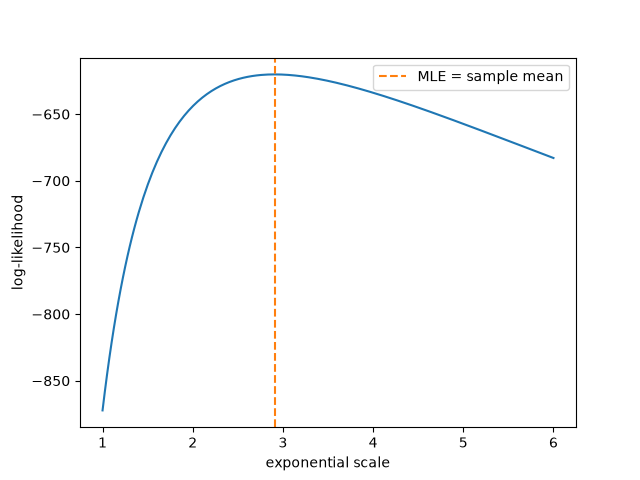
Fits an exponential and a gamma distribution to the same skewed data by maximum likelihood, and plots the exponential model’s log-likelihood as a function of its scale: the curve peaks exactly at the sample mean, the closed-form MLE.

import matplotlib.pyplot as plt
import numpy as np
from scipy import stats

from mathematicskit.statistics import maximum_likelihood_fit

Fitting two candidate models

rng = np.random.default_rng(0)
data = rng.gamma(shape=2.0, scale=1.5, size=300)

expon_fit = maximum_likelihood_fit(data, "expon", floc=0)
gamma_fit = maximum_likelihood_fit(data, "gamma", floc=0)
print(f"exponential: scale={expon_fit.params[1]:.3f} (sample mean {data.mean():.3f}), AIC={expon_fit.aic():.1f}")
print(f"gamma:       shape={gamma_fit.params[0]:.3f}, scale={gamma_fit.params[2]:.3f}, AIC={gamma_fit.aic():.1f}")

exponential: scale=2.908 (sample mean 2.908), AIC=1242.4
gamma:       shape=2.243, scale=1.296, AIC=1154.0

The log-likelihood curve

scales = np.linspace(1.0, 6.0, 200)
loglik = [np.sum(stats.expon.logpdf(data, scale=s)) for s in scales]

fig, ax = plt.subplots()
ax.plot(scales, loglik)
ax.axvline(expon_fit.params[1], color="C1", ls="--", label="MLE = sample mean")
ax.set_xlabel("exponential scale")
ax.set_ylabel("log-likelihood")
ax.legend()

<matplotlib.legend.Legend object at 0x1192f8ec0>