Boyle’s trinomial tree

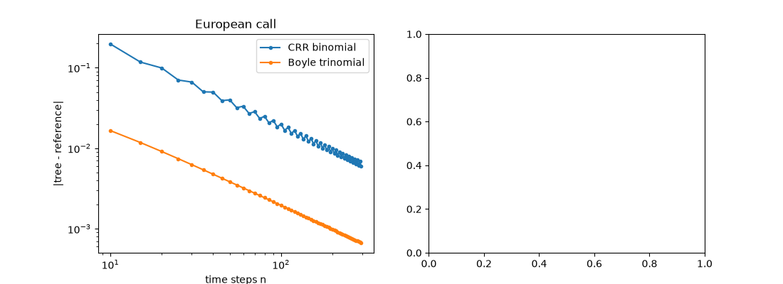
Phelim Boyle (1986) added a third, flat branch to the binomial step. With \(u = e^{\lambda\sigma\sqrt{\Delta t}}\), \(d = 1/u\) and a stretch \(\lambda > 1\), the three probabilities are chosen to match the risk-neutral mean and variance of the next price exactly. The extra branch makes the lattice smoother: for the same number of steps the trinomial tree is usually more accurate than the binomial one.

import matplotlib.pyplot as plt
import numpy as np

from financialkit.options import CRRTree, TrinomialTree, black_scholes_price
from financialkit.options.visualizers import plot_tree_convergence

S, K, T, r, sigma = 100.0, 100.0, 1.0, 0.05, 0.2

Moment matching

tree = TrinomialTree(50)
u, pu, pm, pd = tree.probabilities(T, r, sigma)
dt = T / 50
print(f"p_u = {pu:.4f}, p_m = {pm:.4f}, p_d = {pd:.4f}")
print(f"mean: {pu * u + pm + pd / u:.8f} vs e^(r dt) = {np.exp(r * dt):.8f}")
print(f"second moment: {pu * u**2 + pm + pd / u**2:.8f} vs {np.exp((2 * r + sigma**2) * dt):.8f}")

p_u = 0.3427, p_m = 0.3320, p_d = 0.3254
mean: 1.00100050 vs e^(r dt) = 1.00100050
second moment: 1.00280392 vs 1.00280392

Trinomial vs binomial convergence

exact = black_scholes_price(S, K, T, r, sigma)
steps = np.arange(10, 300, 5)
fig, axes = plt.subplots(1, 2, figsize=(11, 4))
plot_tree_convergence(steps, [CRRTree(n).price(S, K, T, r, sigma).price for n in steps], exact, ax=axes[0], label="CRR binomial")
plot_tree_convergence(steps, [TrinomialTree(n).price(S, K, T, r, sigma).price for n in steps], exact, ax=axes[0], label="Boyle trinomial")
axes[0].set_title("European call")

Text(0.5, 1.0, 'European call')

The stretch parameter

stretches = np.linspace(1.05, 2.0, 20)
errors = [abs(TrinomialTree(100, stretch=lam).price(S, K, T, r, sigma).price - exact) for lam in stretches]
axes[1].semilogy(stretches, errors, "o-")
axes[1].axvline(np.sqrt(1.5), color="k", ls=":", label=r"default $\lambda = \sqrt{3/2}$")
axes[1].set_xlabel(r"stretch $\lambda$")
axes[1].set_ylabel("error with 100 steps")
axes[1].legend()
fig.tight_layout()

plt.show()