Consols and the perpetuity

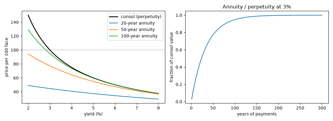
In 1751 Henry Pelham consolidated several British government debts into a single issue of “3 per cent consolidated annuities”, which were never to be repaid: the holder received 3 a year per 100 of face value forever. A perpetuity paying \(P\) is worth \(P/i\) at yield \(i\), so a consol’s price moves inversely with long-term rates and at a 3% yield it trades at par. This script prices consols across yields and compares them with long but finite annuities.

import matplotlib.pyplot as plt
import numpy as np

from financialkit.time_value import annuity_present_value, perpetuity_present_value

Consol prices

for y in (0.025, 0.03, 0.035, 0.05):
    print(f"yield {y:.1%}: consol price {perpetuity_present_value(3.0, y):6.2f}")

yield 2.5%: consol price 120.00
yield 3.0%: consol price 100.00
yield 3.5%: consol price  85.71
yield 5.0%: consol price  60.00

A long annuity is nearly a perpetuity

yields = np.linspace(0.02, 0.08, 121)
fig, axes = plt.subplots(1, 2, figsize=(11, 4))
axes[0].plot(100 * yields, perpetuity_present_value(3.0, yields), "k", lw=2, label="consol (perpetuity)")
for n in (20, 50, 100):
    axes[0].plot(100 * yields, annuity_present_value(3.0, yields, n), label=f"{n}-year annuity")
axes[0].axhline(100.0, color="gray", ls=":")
axes[0].set_xlabel("yield (%)")
axes[0].set_ylabel("price per 100 face")
axes[0].legend()

n = np.arange(1, 301)
axes[1].plot(n, annuity_present_value(3.0, 0.03, n) / perpetuity_present_value(3.0, 0.03))
axes[1].set_xlabel("years of payments")
axes[1].set_ylabel("fraction of consol value")
axes[1].set_title("Annuity / perpetuity at 3%")
fig.tight_layout()

plt.show()