Benford’s law: detecting fabricated figures (1938)

Simon Newcomb noticed in 1881 that the first pages of logarithm tables wore out faster than the last; Frank Benford checked 20,229 numbers from rivers to street addresses in 1938 and found the same law. In data spread over several orders of magnitude, the leading digit is \(d\) with probability

\[P(d) = \log_{10}\left(1 + \frac{1}{d}\right),\]

about 30% for 1 and under 5% for 9: a quantity whose logarithm is spread evenly falls between 1 and 2 more often than between 9 and 10. Products of many random factors, such as payment sizes and prices, follow it. Invented figures rarely do, which is why auditors following Mark Nigrini test reported numbers against the law, and why it has been used to check the trading volumes exchanges report.

import random

import matplotlib.pyplot as plt

import blockchainkit as bk
from blockchainkit.fraud.visualizers import plot_benford

Genuine and invented amounts

Genuine payments: a product of random factors, spread over orders of magnitude. Invented ones: what a person writing “plausible” amounts between 100 and 9,999 might produce, spread evenly.

rng = random.Random(1938)
genuine = [rng.lognormvariate(5, 2) for _ in range(5_000)]
invented = [rng.uniform(100, 9_999) for _ in range(5_000)]
real_test = bk.fraud.benford_test(genuine)
fake_test = bk.fraud.benford_test(invented)
for name, test in (("genuine", real_test), ("invented", fake_test)):
    print(f"{name:9}: chi2 = {test.chi_square:8.1f}, p = {test.p_value:.3g}, {test.conformity}")
assert real_test.conformity in ("close", "acceptable")
assert fake_test.conformity == "nonconformity" and fake_test.p_value < 1e-6

fig, axes = plt.subplots(1, 2, figsize=(11, 4), sharey=True)
plot_benford(real_test, ax=axes[0], label="genuine payments")
plot_benford(fake_test, ax=axes[1], label="invented amounts")
fig.tight_layout()

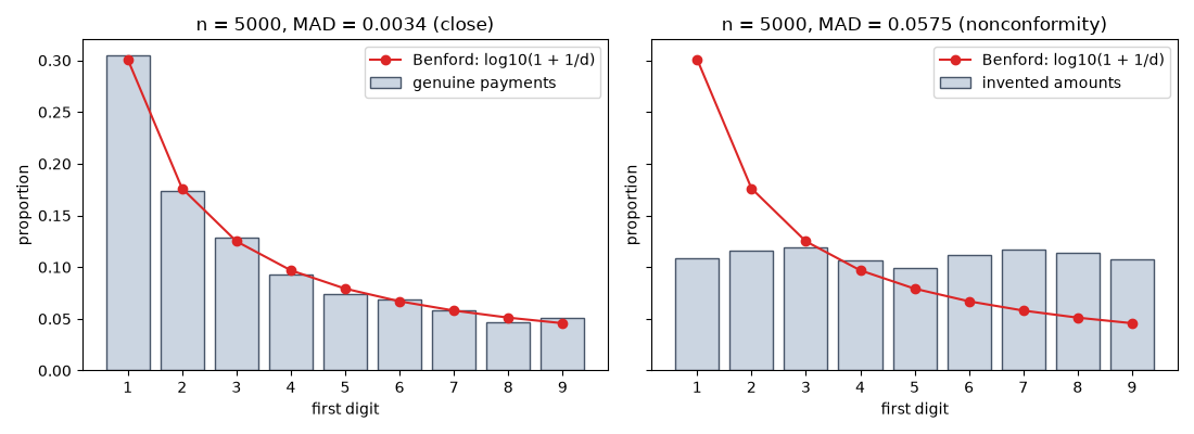
genuine  : chi2 =      8.3, p = 0.403, close
invented : chi2 =   2011.7, p = 0, nonconformity

The chi-square test grows strict with the sample; the deviation does not

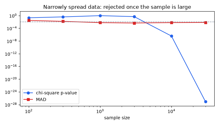
A slight departure from the law fails the chi-square test once the sample is large, while Nigrini’s mean absolute deviation (MAD) stays put.

sizes = [100, 300, 1_000, 3_000, 10_000, 30_000]
slightly_off = [rng.lognormvariate(5, 0.9) for _ in range(sizes[-1])]
p_values = [bk.fraud.benford_test(slightly_off[:n]).p_value for n in sizes]
mads = [bk.fraud.benford_test(slightly_off[:n]).mad for n in sizes]
assert p_values[-1] < 0.01 < p_values[0]

fig, ax = plt.subplots(figsize=(7, 4))
ax.loglog(sizes, p_values, "o-", color="#2563eb", label="chi-square p-value")
ax.loglog(sizes, mads, "s-", color="#dc2626", label="MAD")
ax.axhline(0.01, color="#64748b", linestyle=":")
ax.set(xlabel="sample size", title="Narrowly spread data: rejected once the sample is large")
ax.legend()
fig.tight_layout()

plt.show()

Exercise

The powers of 2 follow Benford’s law. Do the multiples of 7 up to 7,000? Explain the difference with what you know about how each sequence fills orders of magnitude. A worked solution is in Exercises: fraud.