Hanson’s logarithmic market scoring rule (2003)

A prediction market pays 1 for each share of the outcome that happens, so a share’s price reads as a probability. With few traders, an order book is empty and nobody can trade. Hanson’s automated market maker always quotes a price: it keeps the shares \(q_i\) sold of each outcome and charges each trade the change in

\[C(q) = b \ln \sum_i e^{q_i / b}, \qquad p_i = \frac{e^{q_i/b}}{\sum_j e^{q_j/b}}.\]

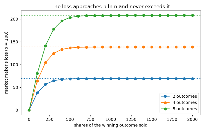
The prices always sum to 1, and the market maker can lose at most \(b \ln n\), the price it pays for the information traders bring. The liquidity \(b\) trades depth against that subsidy.

import matplotlib.pyplot as plt

import blockchainkit as bk

A trader who knows better

The market opens at even odds on two outcomes. A trader who believes outcome 0 has a 90% chance buys until the price reaches 0.9.

fig, ax = plt.subplots(figsize=(7, 4.5))
for b, color in ((50, "#dc2626"), (200, "#2563eb")):
    quantities, shares, prices = [0.0, 0.0], [], []
    paid = 0.0
    while bk.economics.lmsr_prices(quantities, b)[0] < 0.9:
        paid += bk.economics.lmsr_trade(quantities, 0, 5, b)
        quantities[0] += 5
        shares.append(quantities[0])
        prices.append(bk.economics.lmsr_prices(quantities, b)[0])
    print(f"b = {b}: bought {quantities[0]:.0f} shares for {paid:.1f}")
    ax.plot(shares, prices, color=color, label=f"b = {b}")
    if b == 200:
        assert quantities[0] > 4 * 100  # Deeper market, more shares to move the price.

ax.axhline(0.9, color="black", linestyle=":")
ax.set(xlabel="shares of outcome 0 bought", ylabel="price of outcome 0")
ax.set_title("The price follows the purchases")
ax.legend()
fig.tight_layout()

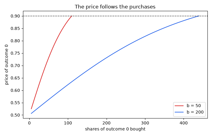
b = 50: bought 110 shares for 80.6
b = 200: bought 440 shares for 322.4

The market maker’s worst case

fig, ax = plt.subplots(figsize=(7, 4.5))
for n in (2, 4, 8):
    losses = []
    for bought in range(0, 2_001, 100):
        quantities = [0.0] * n
        paid = bk.economics.lmsr_trade(quantities, 0, bought, 100)
        losses.append(bought - paid)  # If outcome 0 happens, the maker pays 1 per share.
    bound = bk.economics.lmsr_max_loss(n, 100)
    assert max(losses) <= bound
    ax.plot(range(0, 2_001, 100), losses, "o-", label=f"{n} outcomes")
    ax.axhline(bound, linestyle=":", color=ax.lines[-1].get_color())
ax.set(xlabel="shares of the winning outcome sold", ylabel="market maker's loss (b = 100)")
ax.set_title("The loss approaches b ln n and never exceeds it")
ax.legend()
fig.tight_layout()

plt.show()

Exercise

Two traders disagree: one thinks outcome 0 has a 70% chance, the other 40%. Each trades until the price matches its belief. In which order do they trade to the final price, and what does the market maker pay if outcome 0 happens?