
Breakthroughs in Molecular Structure#
“Chemists were long accustomed to picturing molecules as more or less rigid structures… the more precise our knowledge, the more we realize that this rigidity is not literally true, but the geometric picture remains indispensable.” – paraphrasing the shift, over the century this chronology covers, from bonds drawn as simple connecting lines to bonds understood as electron-pair phenomena with a genuine three-dimensional shape and a discoverable symmetry.
Structural chemistry asks a deceptively simple question: given a
molecular formula, what shape does the molecule actually take, and why?
chemistrykit.structure gathers the computational core of the
answer chemistry has assembled over a century and a half – Lewis
structures and formal charge/oxidation-state bookkeeping, VSEPR geometry
prediction from real 3D electron-domain coordinates, point-group
symmetry classification from direct geometric testing, two
independent routes to a bond order, Kekule-structure enumeration, ring
angle strain, and molecular dipole moments. This chronology traces the
major breakthroughs behind it, from Kekule’s 1865 benzene ring and van’t
Hoff and Le Bel’s 1874 proposal that carbon’s four bonds point toward a
tetrahedron’s corners to the group-theoretic notation this package’s own
character tables still use,
with a pointer to the corresponding implementation in this package at
each stop.
1865 – Kekulé’s Benzene Ring#
August Kekulé had argued in 1858 that carbon is tetravalent and can bond to itself in chains. In 1865 he extended this to the aromatic compounds, proposing that benzene, \(\mathrm{C_6H_6}\), is a closed ring of six carbon atoms joined by alternating single and double bonds, each carbon also carrying one hydrogen. The ring explained why benzene derivatives keep a six-carbon core through many reactions. It also raised a puzzle: with fixed alternating bonds there should be two different 1,2-disubstituted benzenes (substituents across a single bond or across a double bond), but only one is ever found. In 1872 Kekulé proposed that the two alternating arrangements rapidly interconvert, so the six bonds are equivalent on average. That pair of structures is the origin of the later resonance and delocalization pictures of aromatic bonding. In modern graph language, a Kekulé structure is a perfect matching of the carbon skeleton, a set of double bonds that uses every carbon exactly once. Benzene has two, naphthalene three and phenanthrene five, and the count \(K\) is still used as a rough index of aromatic stability.
Implementation:
kekule_structures() enumerates every
Kekulé structure of a conjugated skeleton given its connectivity, and
count_kekule_structures() returns their
number \(K\): 2 for benzene, \(r+1\) for a linear acene with
\(r\) rings, 5 for phenanthrene.
References: A. Kekulé, “Sur la constitution des substances aromatiques,” Bull. Soc. Chim. Paris 3, 98-110 (1865); A. Kekulé, “Ueber einige Condensationsproducte des Aldehyds,” Liebigs Ann. Chem. 162, 77-124 (1872); I. Gutman and S. J. Cyvin, Introduction to the Theory of Benzenoid Hydrocarbons (Springer, Berlin, 1989).
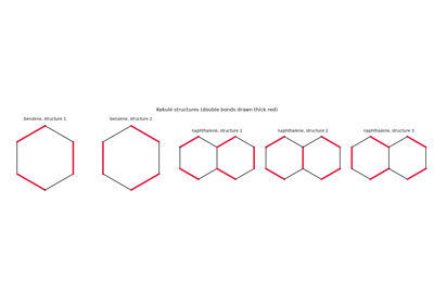
Kekulé’s benzene: enumerating the Kekulé structures of aromatic hydrocarbons
1869 – Mendeleev’s Periodic Table#
Dmitri Mendeleev arranged the 63 elements then known in order of atomic weight and found that their properties (valence, the formulas of their oxides and hydrides, their metallic character) recur periodically. He trusted the periodicity more than the weights. He left gaps for elements not yet discovered and predicted the properties of three of them (gallium, scandium and germanium, all found within 17 years). He also put tellurium before iodine despite its larger atomic weight, because iodine plainly belonged with the halogens. The weight order was not wrong by accident. In 1913 Henry Moseley’s X-ray spectra showed that the true ordering quantity is the nuclear charge, the atomic number \(Z\), and the “inversions” (Ar/K, Co/Ni, Te/I) are simply places where isotopic composition makes a lower-\(Z\) element heavier.
Implementation: chemistrykit.periodic_table.PERIODIC_TABLE
holds all 118 elements with their standard atomic weights,
parse_formula() and
molar_mass() turn formulas into
masses, and PAULING_ELECTRONEGATIVITY
carries one of the periodic properties. The example finds every
atomic-weight inversion against \(Z\) and plots electronegativity’s
periodic rise and fall.
References: D. Mendelejeff, “Über die Beziehungen der Eigenschaften zu den Atomgewichten der Elemente,” Z. Chem. 12, 405-406 (1869); H. G. J. Moseley, “The High-Frequency Spectra of the Elements,” Philos. Mag. 26, 1024-1034 (1913).
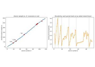
Mendeleev’s periodic table: periodicity and the atomic-weight inversions
1874 – Van’t Hoff and Le Bel’s Tetrahedral Carbon#
Jacobus van’t Hoff and Joseph Le Bel, working independently and publishing within months of each other, proposed the founding result of structural stereochemistry: a carbon atom’s four valence bonds are not confined to a plane but point toward the four vertices of a regular tetrahedron. The proposal explained, at a stroke, a puzzle organic chemists had accumulated data on for years without a structural account – optical isomerism, the existence of two distinct, mirror-image forms of certain compounds that rotate polarized light in opposite directions – by showing that a tetrahedral carbon bonded to four different substituents has no internal mirror symmetry, so its mirror image is a genuinely different, non-superimposable molecule (an enantiomer), while a planar or other non-tetrahedral arrangement would not produce this effect at all. The proposal was not universally welcomed: Hermann Kolbe, a chemist of considerable standing, published a scathing 1877 rebuttal dismissing van’t Hoff’s reasoning as fantastical, unfounded speculation from someone who found the discipline of exact chemical research distasteful – a reaction the tetrahedral-carbon model outlived by well over a century.
Implementation:
domain_positions() generates
exactly this tetrahedral vertex arrangement for a steric number of 4 (the
same construction used for methane in
build_vsepr_molecule()), with
every pair of vertices subtending the exact tetrahedral angle,
109.4712 degrees; building a tetrahedral center with four genuinely
different substituents on top of those same coordinates and testing
whether its mirror image can be superimposed on the original by any
proper rotation is a direct, from-scratch numerical demonstration of
van’t Hoff and Le Bel’s stereochemical claim.
References: J. H. van ‘t Hoff, “Sur les formules de structure dans l’espace,” Archives Néerlandaises des Sciences Exactes et Naturelles 9, 445-454 (1874); J. A. Le Bel, “Sur les relations qui existent entre les formules atomiques des corps organiques et le pouvoir rotatoire de leurs dissolutions,” Bull. Soc. Chim. Fr. 22, 337-347 (1874).
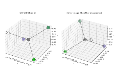
Van’t Hoff and Le Bel’s tetrahedral carbon: chirality from real 3D coordinates
1885 – Baeyer’s Strain Theory#
Adolf von Baeyer, in a paper on polyacetylene compounds, applied van’t Hoff’s tetrahedral carbon to ring compounds. If a carbon’s bonds prefer the tetrahedral angle, \(109.47^\circ\), then a ring whose atoms are forced into a flat polygon, with interior angle \(180^\circ(n-2)/n\), must bend its bonds. Baeyer split the distortion between the two ring bonds at each carbon, giving a strain per bond of
about \(24.7^\circ\) for cyclopropane, \(9.7^\circ\) for cyclobutane and only \(0.7^\circ\) for cyclopentane. This explained why three- and four-membered rings are reactive and easily opened while five- and six-membered rings are so common. Baeyer’s assumption that rings are planar was wrong for larger rings, which his theory predicted to be increasingly strained. Hermann Sachse pointed out in 1890 that cyclohexane can pucker into strain-free “chair” and “boat” forms, an idea confirmed after Ernst Mohr’s 1918 analysis of diamond and decalin, and heats of combustion show cyclohexane to be essentially strain-free. Baeyer’s angle strain survives as one component of the modern ring strain, alongside torsional and transannular strain. Baeyer received the 1905 Nobel Prize in Chemistry, chiefly for his work on dyes and hydroaromatic compounds.
Implementation:
baeyer_angle_strain() computes
\(\delta(n)\) and planar_ring_angle() the
planar ring angle it is measured from, while
chair_cyclohexane_coordinates() builds the
puckered chair with every C-C-C angle exactly tetrahedral, the
counterexample to Baeyer’s planar assumption.
References: A. Baeyer, “Ueber Polyacetylenverbindungen,” Ber. Dtsch. Chem. Ges. 18, 2269-2281 (1885); H. Sachse, “Ueber die geometrischen Isomerien der Hexamethylenderivate,” Ber. Dtsch. Chem. Ges. 23, 1363-1370 (1890); E. L. Eliel and S. H. Wilen, Stereochemistry of Organic Compounds (Wiley, New York, 1994), Ch. 11.
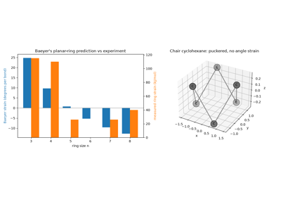
Baeyer’s strain theory: angle strain in planar cycloalkane rings
1891 – Schoenflies and Point-Group Notation#
Building on Johann Hessel’s little-noticed 1830 enumeration of the 32 crystallographic point groups and Auguste Bravais’s independent 1849 rediscovery of them, Arthur Schoenflies – working in close (and at times competitive) parallel with the Russian crystallographer Evgraf Fedorov – gave crystal and molecular symmetry a systematic algebraic notation in his 1891 Krystallsysteme und Krystallstructur: a symmetry group is named by its defining generators, a principal rotation axis \(C_n\), the dihedral \(D_n\) families with perpendicular \(C_2\) axes, the mirror-plane refinements \(\sigma_h\)/ \(\sigma_v\)/\(\sigma_d\), an inversion center \(i\), and the improper-rotation axes \(S_n\), combined into symbols like \(C_{2v}\), \(D_{3h}\), or \(T_d\). Where Fedorov’s contemporaneous, independently derived classification of the 230 space groups is the crystallographer’s standard reference today, it is specifically Schoenflies’s point-group symbols – built for the finite, non-translational symmetry of an individual molecule or crystal motif rather than an infinite periodic lattice – that became, and remains, the universal notation for molecular symmetry in chemistry.
Implementation: every point group
determine_point_group()
returns – "C2v", "Td", "D_inf_h", and so on – is spelled in
exactly Schoenflies’s own notation, and
PointGroupCharacterTable
together with CHARACTER_TABLES
tabulate the standard character tables under that same naming scheme.
References: A. Schoenflies, Krystallsysteme und Krystallstructur (Teubner, Leipzig, 1891). A book, not a journal article – there is no DOI to cite. The parallel priority of Fedorov’s independent space-group derivation (published in Russian in the same period) is well documented in the crystallographic literature but not itself the source of the point-group notation this package uses.
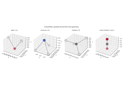
Schoenflies point-group symbols for water, ammonia, methane, and carbon dioxide
1893 – Werner’s Coordination Theory#
Alfred Werner proposed, in “Beitrag zur Konstitution anorganischer Verbindungen,” that a transition-metal complex’s ligands occupy fixed geometric positions around the central metal – six ligands at the vertices of an octahedron, or four at the corners of a square plane or a tetrahedron – fundamentally distinct from and independent of the metal’s own ordinary ionic valence. At a time decades before X-ray crystallography or any other technique could directly image a molecule’s three-dimensional shape, Werner supported this entirely through painstaking indirect evidence: counting the number of distinct isomers a given complex could be resolved into, and showing that only his proposed octahedral (rather than, say, hexagonal-planar) geometry predicted the correct number of isomers for compound after compound. He was awarded the 1913 Nobel Prize in Chemistry for this work, becoming the first inorganic chemist to receive it. Werner’s octahedral six-coordination is not confined to transition-metal complexes; it is exactly the electron- domain arrangement VSEPR theory (see 1940-1970, below) later predicted from first principles for any steric-number-6 center, transition metal or main-group alike.
Connection: domain_positions()
with steric_number=6 generates precisely Werner’s proposed
octahedral vertex arrangement, and
determine_point_group()
classifies a regular six-coordinate structure built on those vertices as
\(O_h\) – recovering, by direct geometric symmetry testing rather
than isomer-counting, the same octahedral picture Werner had to infer
indirectly; chemistrykit.structure.systems.point_group’s recently
fixed handling of the four body-diagonal \(C_3\) axes an
\(O_h\) structure requires (see the module’s candidate-axis
docstring) is exactly what makes that classification correct for a
genuinely six-coordinate, cardinal-axis-ligand geometry.
References: A. Werner, “Beitrag zur Konstitution anorganischer Verbindungen,” Z. Anorg. Chem. 3, 267-330 (1893).
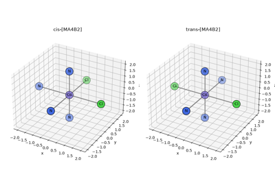
Werner’s coordination theory: counting isomers to prove the octahedron
1912 – Debye’s Permanent Dipole Moments#
Peter Debye explained why the dielectric constant of some gases falls as the temperature rises while that of others hardly changes. Molecules of the first kind carry a permanent electric dipole moment, \(\boldsymbol\mu = \sum_i q_i \mathbf r_i\) for charges \(q_i\) at positions \(\mathbf r_i\), which an applied field partly aligns against thermal disorder. This adds a term \(\mu^2/3k_BT\) to the molecular polarizability, so the dipole moment can be read off the slope of polarization against \(1/T\). Measured moments became a direct test of molecular shape. A molecular dipole is the vector sum of its bond dipoles, so symmetric shapes cancel: linear \(\mathrm{CO_2}\), trigonal planar \(\mathrm{BF_3}\) and tetrahedral \(\mathrm{CH_4}\) have no moment, while bent water (1.85 D) and pyramidal ammonia do. Only molecules in the point groups \(C_n\), \(C_{nv}\) and \(C_s\) can be polar. Debye’s 1929 monograph Polar Molecules collected the method, and he received the 1936 Nobel Prize in Chemistry in part for this work. The unit of dipole moment, the debye (\(10^{-18}\) esu cm, about 0.208 e Å), is named after him.
Implementation:
dipole_moment() computes
\(\sum_i q_i\mathbf r_i\) in debye from partial charges and
coordinates, bond_dipole_sum() adds bond
dipoles as vectors, and E_ANGSTROM_IN_DEBYE gives the unit conversion
(4.803 D per e Å).
References: P. Debye, “Einige Resultate einer kinetischen Theorie der Isolatoren,” Phys. Z. 13, 97-100 (1912); P. Debye, Polar Molecules (Chemical Catalog Company, New York, 1929).
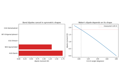
Debye’s permanent dipole moments: polar and nonpolar molecules from geometry
1916 – Lewis’s Shared Electron Pair#
Gilbert N. Lewis proposed, in “The Atom and the Molecule,” that a covalent bond is nothing more or less than a pair of electrons shared between two atoms – replacing the vaguer nineteenth-century notion of “valence” with a concrete, countable electronic picture, and introducing the dot-and-line notation (a Lewis structure) still taught as the first step of structural chemistry today. Lewis’s octet rule – that atoms tend toward an arrangement of eight shared and unshared valence electrons, mimicking a noble gas’s stable configuration – gave chemists a systematic bookkeeping procedure for predicting which bonding patterns are reasonable at all, and formal charge became the natural tool for comparing among multiple electronically valid Lewis structures for the same molecule: split every bonding pair evenly between its two atoms, regardless of which is more electronegative, and compare the resulting charge on each atom to what the free, neutral atom would have.
Implementation:
chemistrykit.structure.systems.lewis.LewisStructure represents
exactly this dot-and-line bookkeeping – element symbols, bond orders,
and lone-pair counts – and its
formal_charges()
computes the formula above directly;
total_formal_charge()
implements the standard self-consistency check that a valid Lewis
structure’s formal charges must sum to the molecule’s actual net charge.
References: G. N. Lewis, “The Atom and the Molecule,” J. Am. Chem. Soc. 38, 762-785 (1916).
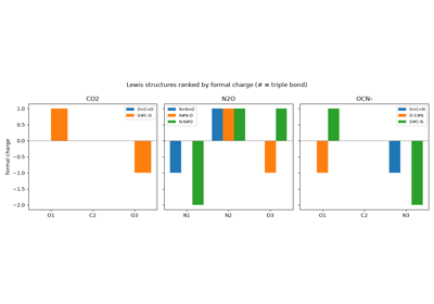
Lewis’s shared electron pair: choosing between Lewis structures by formal charge
1916 – Kossel’s Ionic Bond and the Two Extremes of Bond Polarity#
In the same year as Lewis’s covalent-bond paper, and entirely independently, Walther Kossel proposed the complementary extreme: a bond forms when one atom transfers an electron (or several) outright to another, each ending up with a noble-gas electron configuration as a charged ion, held together purely by electrostatic (Coulombic) attraction rather than any shared electron pair. Real bonds, of course, sit somewhere between Kossel’s fully ionic picture and Lewis’s fully covalent, evenly shared one – the actual electron distribution shifts toward whichever atom is more electronegative, but rarely transfers completely – and the two men’s independent, same-year papers are naturally read today as marking out the two idealized limits that real, partially polar bonds interpolate between. Oxidation state is the electron-bookkeeping convention built on Kossel’s ionic extreme, exactly as formal charge is built on Lewis’s evenly-shared one: assign every bonding pair entirely to its more electronegative partner (split evenly only for a homonuclear bond, where neither atom has a legitimate claim to more), and compare the resulting electron count to the free atom’s.
Implementation:
oxidation_states()
implements exactly this fully-ionic-limit bookkeeping, using Pauling-scale
electronegativities from chemistrykit.periodic_table.electronegativity()
to decide, bond by bond, which atom is assigned the shared electrons –
the direct computational counterpart of
formal_charges()’s
evenly-split, Lewis-style convention on the very same
LewisStructure.
References: W. Kossel, “Über Molekülbildung als Frage des Atombaus,” Ann. Phys. 354, 229-362 (1916).
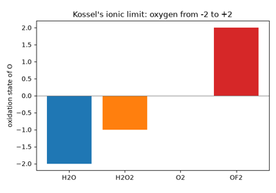
Kossel’s ionic bond: oxidation states as the fully ionic limit
1929 – Bethe’s Crystal-Field Theory and Group Theory Enters Chemistry#
Hans Bethe’s “Termaufspaltung in Kristallen” asked what happens to a free ion’s electronic energy levels once it is placed inside a crystal (or, in the molecular reading adopted a few years later, at the center of a coordination complex’s ligand arrangement): the surrounding electrostatic field, no longer spherically symmetric but only as symmetric as the local point group, splits levels that were degenerate in the free ion into separate sub-levels, in a pattern group theory alone – without any detailed calculation of the field’s actual strength – can predict completely. Bethe’s paper was the first systematic demonstration that a molecule or crystal site’s point-group symmetry, treated by its formal group-theoretic machinery (irreducible representations, character tables), directly constrains which physical splittings and which spectroscopic transitions are allowed, independent of any detail of the interatomic forces involved – the origin of what would later be called crystal-field and ligand-field theory, and the entry point of formal group theory into chemistry more broadly. Applied to a six-coordinate octahedral complex, Bethe’s analysis shows a transition-metal ion’s five formerly degenerate d-orbitals split into two sets transforming as the octahedral group’s \(e_g\) and \(t_{2g}\) irreducible representations – the single most-cited result of crystal-field theory, and still the first thing taught in any treatment of transition-metal complex color and magnetism.
Implementation:
get_character_table()
returns exactly the \(O_h\) character table Bethe’s analysis is built
on, with PointGroupCharacterTable’s
Eg/T2g irreps (and their tabulated dimensions, 2 and 3
respectively) the same labels crystal-field theory attaches to the split
d-orbital sets – the group-theoretic classification machinery this
package implements is precisely the tool Bethe’s theory needs, applied
here to a concrete \(O_h\) structure (sulfur hexafluoride) rather
than a transition-metal complex, since chemistrykit.structure
does not model transition-metal electronic structure directly.
reduce() carries out
Bethe’s reduction itself: fed the characters of the five d orbitals under
the \(O_h\) operations, it returns \(E_g + T_{2g}\).
References: H. Bethe, “Termaufspaltung in Kristallen,” Ann. Phys. 395, 133-208 (1929).
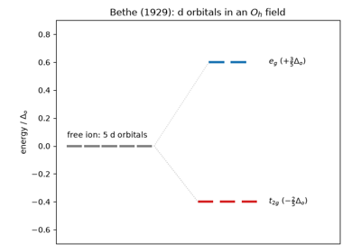
Bethe’s crystal-field splitting: d orbitals in an octahedral field
1932 – Pauling’s Electronegativity Scale#
Linus Pauling, in the fourth installment of his landmark “The Nature of the Chemical Bond” series, noticed that a bond between two different elements is almost always stronger than the average of the two corresponding homonuclear bonds’ strengths – an “extra ionic energy” he attributed to the bond’s partial ionic character, and which he showed could be used to define a self-consistent, quantitative scale of each element’s tendency to attract shared electrons: electronegativity. The resulting Pauling scale (fluorine assigned the highest value, 3.98, by convention) let chemists move past qualitative, ad hoc statements about which atoms “want” electrons more and instead compute or measure the ionic character of a specific bond directly from the electronegativity difference between its two atoms – one part of Pauling’s broader program in The Nature of the Chemical Bond (collected as a monograph in 1939), which also included the hybridization and resonance concepts that gave quantum mechanics a usable, qualitative vocabulary for practicing chemists. Pauling was awarded the 1954 Nobel Prize in Chemistry for this body of work.
Implementation:
chemistrykit.periodic_table.electronegativity() tabulates exactly
the Pauling scale values this paper introduced, and
oxidation_states()
(see 1916, above) uses them directly to decide, bond by bond, which atom
is the more electronegative partner – the same electronegativity
comparison Pauling’s own ionic-character argument is built on.
pauling_electronegativity_difference()
reproduces Pauling’s original construction, turning the extra ionic
energy of an A-B bond (from bond dissociation energies) into
\(|\chi_A - \chi_B|\).
References: L. Pauling, “The Nature of the Chemical Bond. IV. The Energy of Single Bonds and the Relative Electronegativity of Atoms,” J. Am. Chem. Soc. 54, 3570-3582 (1932).
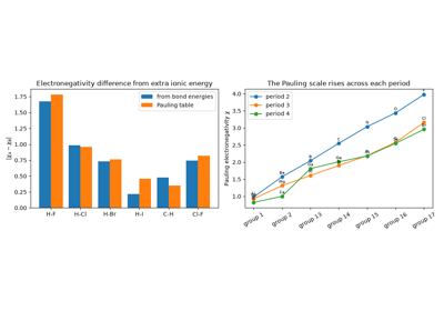
Pauling’s electronegativity scale from bond energies
1939 – Coulson’s Molecular-Orbital Bond Order#
Charles Coulson, applying Erich Huckel’s decade-old pi-electron molecular-orbital theory to conjugated and aromatic hydrocarbons, defined a bond order directly from the resulting molecular-orbital coefficients rather than from any experimentally measured bond length:
summed over occupied molecular orbitals \(k\) weighted by their electron occupation \(n_k\). Applied to benzene, this gives a pi bond order of exactly 2/3 for every carbon-carbon bond – neither the single nor the double bond a single Kekule structure would suggest, but the delocalized average consistent with all six ring bonds being experimentally identical in length. The Coulson bond order gave chemists a genuinely independent, first-principles-electronic-structure route to the same fractional-bond-order concept Pauling’s contemporary empirical length correlation (see 1947, below) reached from measured geometry alone – two unrelated methods converging on the same answer for benzene’s bonding is, still today, one of the standard textbook demonstrations that aromatic delocalization is real rather than a mere notational convenience.
Implementation:
coulson_pi_bond_order()
implements exactly this formula, computed directly from
chemistrykit.quantum.systems.huckel.HuckelSystem’s molecular-
orbital coefficients – reusing chemistrykit.quantum’s existing
Huckel-theory machinery rather than re-deriving it, since Coulson’s bond
order is a direct property of the Huckel molecular orbitals themselves.
References: C. A. Coulson, “The Electronic Structure of Some Polyenes and Aromatic Molecules. VII. Bonds of Fractional Order by the Molecular Orbital Method,” Proc. R. Soc. Lond. A 169, 413-428 (1939).
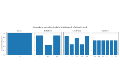
Coulson’s molecular-orbital bond order in butadiene, hexatriene, and benzene
1940 – 1970 – Sidgwick, Powell, Gillespie, and Nyholm: VSEPR Theory#
Nevil Sidgwick and Herbert Powell’s 1940 Bakerian Lecture, “Stereochemical Types and Valency Groups,” first proposed systematically that a central atom’s molecular shape is governed simply by the number of electron pairs (bonding and lone) in its valence shell arranging themselves to minimize mutual repulsion, treating both kinds of pair as occupying comparable, roughly equivalent regions of space around the nucleus. Ronald Gillespie and Ronald Nyholm developed the idea into a complete, quantitatively predictive theory in their 1957 “Inorganic Stereochemistry” – crucially adding the refinement that a lone pair, being more diffuse and held closer to the nucleus than a bonding pair, repels its neighbors more strongly, systematically compressing the bond angles around it relative to the idealized polyhedron (real ammonia’s 106.7-degree H-N-H angle and water’s 104.5-degree H-O-H angle, both compressed from a parent tetrahedron’s 109.47 degrees, are the textbook illustrations). Gillespie gave the resulting model its now-standard pedagogical form, and its name, in a widely read 1970 article. For a steric number of \(N\) electron domains, the model predicts one of five idealized parent polyhedra – linear, trigonal planar, tetrahedral, trigonal bipyramidal, octahedral – with lone pairs then displacing specific vertices to produce the full catalogue of real molecular shapes (bent, trigonal pyramidal, seesaw, T-shaped, square pyramidal, square planar, and more).
Implementation:
domain_positions() generates
the five idealized polyhedra’s genuine 3D vertex coordinates directly
from their defining symmetry (not a shape-name lookup table), and
VSEPRGeometry together with
build_vsepr_molecule()
implement Gillespie and Nyholm’s lone-pair-placement rule – lone pairs
preferentially occupy the least sterically crowded available positions –
reproducing water’s bent AX2E2 shape, sulfur tetrafluoride’s seesaw
AX4E1 shape, and xenon tetrafluoride’s square-planar AX4E2 shape exactly
this way, with AXE_SHAPE_NAMES
tabulating Gillespie’s own AXE nomenclature for each combination.
References: N. V. Sidgwick and H. M. Powell, “Bakerian Lecture. Stereochemical Types and Valency Groups,” Proc. R. Soc. Lond. A 176, 153-180 (1940); R. J. Gillespie and R. S. Nyholm, “Inorganic Stereochemistry,” Q. Rev. Chem. Soc. 11, 339-380 (1957); R. J. Gillespie, “The Electron-Pair Repulsion Model for Molecular Geometry,” J. Chem. Educ. 47, 18-23 (1970).
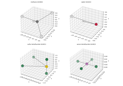
VSEPR geometry prediction: from steric number to real 3D coordinates
1947 – Pauling’s Bond-Order/Bond-Length Correlation#
Linus Pauling observed empirically that, within a family of similar bonds (carbon-carbon bonds, most famously), a bond’s length shrinks in a consistent, logarithmic way as its bond order increases:
with \(D(1)\) a reference single-bond length and \(c\) an empirically fitted, bond-type-specific constant (Pauling’s own value for carbon-carbon bonds, 0.71 angstrom, which puts the double and triple bonds at 1.33 and 1.20 angstrom). Inverting the relation lets a measured, non-integer bond length be converted directly into an estimated, generally non-integer bond order – applied to benzene’s carbon-carbon bond length of 1.397 angstrom (intermediate between ethane’s 1.54-angstrom single bond and ethylene’s 1.34-angstrom double bond), the correlation predicts a bond order between 1 and 2, an entirely independent empirical confirmation of the same delocalized-bonding picture Coulson’s molecular-orbital theory (see 1939, above) reaches from the electronic structure side rather than the geometric one.
Implementation:
bond_order_from_length() and
its exact inverse
bond_length_from_order()
implement exactly this formula, with
PAULING_C_C_CONSTANT
Pauling’s own carbon-carbon correlation constant (flagged explicitly in
the module as needing re-fitting for any other bond type, which this
module does not tabulate).
References: L. Pauling, “Atomic Radii and Interatomic Distances in Metals,” J. Am. Chem. Soc. 69, 542-553 (1947).
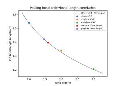
Pauling’s bond-order and bond-length correlation for carbon-carbon bonds
1955 – Mulliken’s Notation for Molecular Term Symbols#
As group-theoretic methods spread through molecular spectroscopy in the decades after Bethe’s crystal-field paper, different research groups had adopted inconsistent, sometimes conflicting labels for a molecule’s irreducible representations – an obstacle to comparing results across the growing literature. Robert Mulliken’s 1955 “Report on Notation for the Spectra of Polyatomic Molecules,” prepared for and endorsed by the Joint Commission for Spectroscopy, standardized the convention still used universally today: a one-dimensional representation is labeled \(A\) (symmetric under the principal rotation) or \(B\) (antisymmetric under it), a two-dimensional one \(E\), and a three-dimensional one \(T\), with a subscript \(g\)/\(u\) marking symmetric/antisymmetric behavior under inversion (for centrosymmetric groups) and numeric subscripts distinguishing multiple representations that would otherwise share the same letter. Mulliken received the 1966 Nobel Prize in Chemistry for his broader body of work on chemical bonds and the electronic structure of molecules, of which this notational standardization was a comparatively small, but enduringly practical, contribution.
Implementation: every irreducible-representation label in
chemistrykit.structure.systems.point_group.CHARACTER_TABLES –
"A1", "B2", "Eg", "T2u", and so on, for every point group
this package tabulates – is spelled in exactly Mulliken’s notation, and
character()
looks up a specific character by exactly these labels.
References: R. S. Mulliken, “Report on Notation for the Spectra of Polyatomic Molecules,” J. Chem. Phys. 23, 1997-2011 (1955).
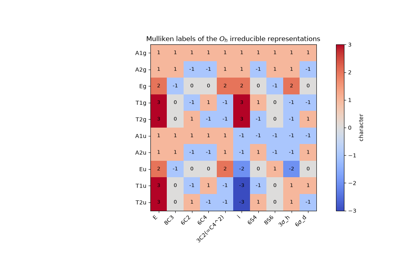
Mulliken symbols: reading the labels of irreducible representations
1969 – Musher and Hypervalent Bonding#
Molecules like sulfur hexafluoride, phosphorus pentachloride, and xenon tetrafluoride pose a puzzle Lewis’s 1916 octet rule (see above) does not obviously resolve: their central atoms are bonded to five or six neighbors, apparently exceeding the eight-electron limit an s-and-p valence shell should allow. For decades the standard explanation invoked participation of the central atom’s empty d-orbitals to accommodate the extra bonds; James Musher’s 1969 review, “The Chemistry of Hypervalent Molecules,” gave the whole class of such species its now-standard name and argued for treating them as a coherent structural category in their own right, distinct from ordinary (octet-obeying) molecules – a framing that anticipated, and helped motivate, the modern three-center-four-electron bonding picture that later largely displaced the d-orbital explanation, which quantitative calculations have since shown contributes only marginally to real hypervalent bonding. Crucially, VSEPR’s electron-domain counting (see 1940-1970, above) never depended on which bonding picture – d-orbital participation, three-center-four-electron bonds, or otherwise – turned out to be correct: it predicts a hypervalent center’s geometry correctly regardless of the underlying electronic mechanism, simply by counting domains.
Connection: domain_positions()
generates the five- and six-domain polyhedra (trigonal bipyramidal,
octahedral) that every hypervalent AX5/AX6-type molecule this package’s
own gallery builds – sulfur tetrafluoride, xenon tetrafluoride, sulfur
hexafluoride – relies on, entirely independent of any specific bonding-
model explanation for how a main-group atom accommodates more than four
electron domains at all.
References: J. I. Musher, “The Chemistry of Hypervalent Molecules,” Angew. Chem. Int. Ed. 8, 54-68 (1969).
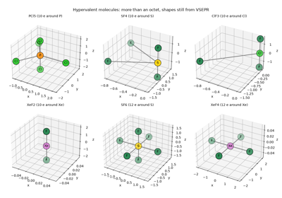
Musher’s hypervalent molecules: main-group centres beyond the octet