
Breakthroughs in Quantum Chemistry#
“The underlying physical laws necessary for the mathematical theory of a large part of physics and the whole of chemistry are thus completely known, and the difficulty is only that the exact application of these laws leads to equations much too complicated to be soluble.” – P. A. M. Dirac, Proc. R. Soc. Lond. A 123, 714-733 (1929)
Dirac’s remark, made barely three years after Schrodinger’s wave equation
first appeared, is also this package’s mission statement in miniature:
chemistrykit.quantum is a chronicle of exactly the approximations
chemists built to make Dirac’s “equations much too complicated to be
soluble” soluble anyway – valence-bond and molecular-orbital pictures of
the covalent bond, Huckel’s drastic but durable simplification of
conjugated pi systems, and the Gaussian-basis variational machinery that,
in Roothaan and Hall’s hands, turned Hartree-Fock theory from a
principle into a computer program. A handful of results below (the
Schrodinger equation itself, foremost) are shared ancestry with
physicskit.quantum’s own general treatment of quantum mechanics
and are only briefly set the scene here; the chronology’s real subject is
the distinct cast of chemists who spent the following quarter-century
turning that equation into a working theory of the chemical bond. Each
stop below is paired with the corresponding implementation in this
package.
1916 – Lewis’s Shared-Electron-Pair Theory of the Covalent Bond#
Nine years before Heisenberg and Schrodinger gave quantum mechanics its mathematical form, the American chemist Gilbert N. Lewis proposed a purely structural idea that would turn out to anticipate it: a covalent bond between two atoms is a shared pair of electrons, jointly holding both nuclei together, with each atom’s stable configuration built around completing an outer octet of such shared and unshared pairs. Lewis’s theory had no dynamics, no wave equation, and no way to compute a bond energy from first principles – it was pure bookkeeping, dots and lines on a page – but it correctly identified the conceptual unit later theories would need to explain quantum-mechanically: not a bond as a classical force between charges, but a bond as two electrons of opposed spin, delocalized between (or, in valence-bond language, exchanged between) two nuclei. Every quantum-mechanical theory of bonding below, valence-bond and molecular-orbital alike, is in this sense an attempt to derive Lewis’s electron pair from the Schrodinger equation rather than replace it.
Connection: this package has no direct “Lewis structure” implementation
– the entire point of the theories below is to go beyond dots-and-lines
bookkeeping – but Lewis’s electron-pairing rule reappears, quantum-
mechanically justified, wherever two electrons of opposite spin are
placed together in the same spatial orbital: two electrons filling
chemistrykit.quantum.systems.hartree_fock.H2PlusVariational’s
bonding molecular orbital (rather than one each in the bonding and
antibonding orbitals) is exactly a quantum-mechanical shared electron
pair, and
pi_electron_energy()’s
“two electrons per orbital, lowest energy first” Aufbau filling rule is
the same pairing principle applied systematically across an entire
conjugated pi system.
References: G. N. Lewis, “The Atom and the Molecule,” J. Am. Chem. Soc. 38, 762-785 (1916).
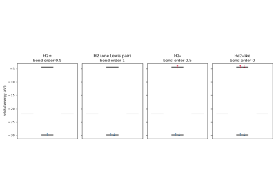
Lewis’s shared electron pair: two opposite-spin electrons in one bonding orbital
1926 – Schrodinger’s Wave Mechanics: the Equation, the Atom, and Perturbation Theory#
In a single extraordinary year, Erwin Schrodinger published a four-part series, “Quantisierung als Eigenwertproblem” (“Quantization as an Eigenvalue Problem”), that gave quantum theory the mathematical form it has kept ever since. The first two parts introduced the time-independent wave equation and solved it exactly for the two textbook systems every subsequent quantum-chemistry course still opens with – the harmonic oscillator and, most consequentially for chemistry, the hydrogen atom, whose energy levels the new wave mechanics reproduced exactly, without Bohr’s ad hoc quantization postulates and with a clean physical interpretation (Born’s, shortly afterward) of what \(|\psi|^2\) actually means.
The equation’s exact solvability was itself a rarity, though, and Schrodinger’s third installment addressed what to do about every case where it fails: adapting a perturbative technique from Lord Rayleigh’s 19th-century classical theory of coupled vibrating systems, he showed how to build an approximate correction to a known solution’s energy and wavefunction directly from the difference between the true Hamiltonian and a solvable one – Rayleigh-Schrodinger perturbation theory, applied in that same paper to the Stark effect on the hydrogen spectrum. It remains, a full century later, the standard first resort whenever a real molecule’s Hamiltonian is “close to” some exactly solvable model but not equal to it – a real anharmonic bond potential and its own harmonic approximation, prototypically.
Implementation: chemistrykit.quantum.systems.hydrogenlike.HydrogenLikeAtom
solves exactly this equation’s hydrogen-atom special case, reproducing
the textbook 13.6 eV ground state to three figures and, with the true
electron-nucleus reduced mass, to five or six; the closely related exact
solutions for a particle confined to a box
(ParticleInBox1D,
ParticleInBox3D)
are the same equation applied to the other textbook potential this
package builds on. Rayleigh-Schrodinger perturbation theory itself is
implemented in chemistrykit.quantum.systems.perturbation:
quartic_perturbation_first_order_correction()
gives the first-order energy shift from a quartic anharmonic term
directly from the harmonic-oscillator ladder-operator matrix elements
(position_operator_matrix()),
checked in turn against
anharmonic_energy_levels()’s
exact numerical diagonalization of the same truncated problem.
References: E. Schrodinger, “Quantisierung als Eigenwertproblem (Erste Mitteilung),” Ann. Phys. 79, 361-376 (1926); “(Zweite Mitteilung),” Ann. Phys. 79, 489-527 (1926); “(Dritte Mitteilung: Storungstheorie, mit Anwendung auf den Starkeffekt der Balmerlinien),” Ann. Phys. 80, 437-490 (1926) (pagination as commonly cited in secondary literature for this well-known four-part series; not independently re-verified against the original Annalen der Physik volumes).
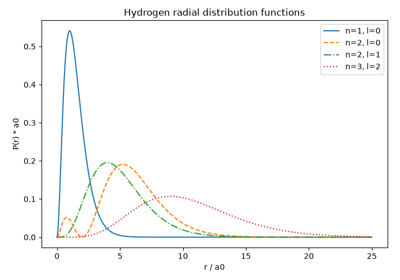
Schrodinger’s hydrogen atom: radial wavefunctions and orbital energies
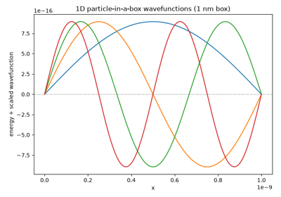
Solving Schrodinger’s equation for a particle in a box
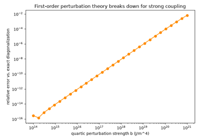
Rayleigh-Schrodinger perturbation theory vs. exact diagonalization for the quartic oscillator
1926 – Dennison and the Quantum Theory of Molecular Rotation#
David Dennison applied Schrodinger’s brand-new wave equation to a problem with a genuinely chemical payoff: a diatomic molecule’s end-over- end rotation, modeled as a rigid rotor with a fixed bond length. Solving the angular Schrodinger equation gives energy levels \(E_J\propto J(J+1)\) – not evenly spaced, unlike a harmonic oscillator’s vibrational ladder, but spaced with a gap that itself grows linearly with J – each level \((2J+1)\)-fold degenerate, and, under the \(\Delta J=\pm1\) selection rule that a rotating polar molecule’s transitions obey, giving evenly spaced pure-rotational absorption lines in the microwave region: the first quantitative theoretical basis for rotational (microwave) spectroscopy as a chemical tool for measuring bond lengths directly. Dennison returned to the rigid rotor the following year with an even more striking chemical consequence: hydrogen gas’s specific heat, anomalously low at cryogenic temperature compared to the classical rigid-rotor prediction, is explained once the two nuclear-spin species of H2 – para-hydrogen (even J only) and ortho-hydrogen (odd J only) – are recognized as behaving as two separate gases with different rotational partition functions, a genuinely quantum-statistical effect of nuclear spin on a bulk thermodynamic property.
Implementation: chemistrykit.quantum.systems.rigid_rotor.RigidRotor
implements exactly this spectrum,
degeneracy()
gives \(g_J\), and
transition_energy()
confirms the evenly-spaced-by-\(2B\) microwave selection-rule
prediction directly;
from_diatomic()
builds the model straight from a real molecule’s atomic masses and bond
length, exactly the direction (bond length from measured microwave
spectrum) rotational spectroscopy runs in practice.
References: D. M. Dennison, “The Rotation of Molecules,” Phys. Rev. 28, 318-333 (1926); D. M. Dennison, “A Note on the Specific Heat of the Hydrogen Molecule,” Proc. R. Soc. Lond. A 115, 483-486 (1927).
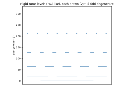
Dennison’s rigid rotor: rotational levels and the microwave spectrum
1927 – Born and Oppenheimer’s Separation of Nuclear and Electronic Motion#
Max Born and J. Robert Oppenheimer noticed that the full molecular Schrodinger equation – nuclei and electrons together, every particle’s kinetic and potential energy coupled to every other’s – is, in practice, far more tractable than it looks, because a proton is roughly 1,800 times heavier than an electron, so the nuclei move enormously more slowly. To the fast-moving electrons, the nuclei look essentially frozen in place at any given instant; to the slow-moving nuclei, the electrons’ rapid motion averages out into a smooth, effective potential-energy surface that depends only on the nuclear positions. Formalizing this separation (rigorously, as an expansion in the fourth root of the electron-to-nuclear mass ratio) lets the intractable coupled problem be solved in two much smaller stages instead of one enormous one: first solve the electronic Schrodinger equation with the nuclei clamped at some fixed geometry, to get an electronic energy that is itself a function of that geometry; then solve a separate, purely nuclear Schrodinger equation – vibration, rotation – using that electronic energy curve as the potential the nuclei move in. This clamped-nuclei approximation is not a minor computational convenience but the conceptual foundation the entire rest of this package’s electronic-structure and nuclear-motion machinery rests on: without it, “the” energy of a molecule at “a” bond length – the single number every potential-energy curve, force constant, and equilibrium geometry in this subpackage is built from – would not even be a well-defined quantity, since a fully coupled treatment has no notion of a fixed nuclear geometry to attach an electronic energy to in the first place.
Connection: chemistrykit.quantum.systems.hartree_fock.H2PlusVariational
takes its two protons’ separation as a fixed input parameter,
bond_length, and solves only the electronic problem at that clamped
geometry – exactly the Born-Oppenheimer electronic step, with the second,
nuclear-motion step left to the separate
RigidRotor (above) and
MorseOscillator
(below) models, each of which likewise takes a fixed equilibrium bond
length or force constant as given rather than solving for the nuclei and
electrons together; the same clamped-nuclei logic underlies the isotope
shift discussion in Breakthroughs in Spectroscopy, where a
heavier nucleus changes a molecule’s rotational constant while leaving
its (electronically determined) bond length untouched.
References: M. Born and R. Oppenheimer, “Zur Quantentheorie der Molekeln,” Ann. Phys. 389, 457-484 (1927).
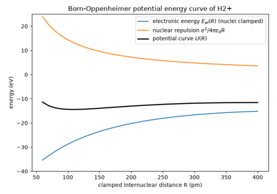
Born-Oppenheimer clamped-nuclei potential curve of H2+
1927 – Heitler and London’s Quantum-Mechanical Treatment of H2#
Walter Heitler and Fritz London’s treatment of the hydrogen molecule is routinely credited as the birth of quantum chemistry as a distinct field, because it was the first calculation to show, from the Schrodinger equation alone and with no chemistry assumed in advance, that two neutral hydrogen atoms genuinely attract each other into a stable bond – putting Lewis’s 1916 shared electron pair on quantum-mechanical footing eleven years after the fact. Their trial wavefunction combined each atom’s exact 1s orbital two ways: symmetrically (the spatial part unchanged under swapping the two electrons) and antisymmetrically. Because the total two-electron wavefunction must be antisymmetric overall (Pauli), the spatially symmetric combination pairs with an antisymmetric (singlet) spin state – opposite-spin electrons, exactly Lewis’s shared pair – and Heitler and London’s variational calculation showed that combination alone lowers the energy below that of two separated atoms, while the antisymmetric spatial (triplet) combination raises it: a real chemical bond, or its absence, falling directly out of the mathematics of identical-particle exchange rather than being assumed.
Implementation: the full two-electron exchange and Coulomb integrals
Heitler and London’s original calculation needed are beyond this
package’s scope (chemistrykit.quantum.utils.basis_sets implements
only the one-electron integrals
H2PlusVariational
needs for H2+), but the same qualitative mechanism – a spatially symmetric
combination of two atomic-like orbitals building up electron density
between the nuclei (lowering the energy), and the antisymmetric
combination depleting it there (raising the energy) – is exactly what a
dedicated example built for this history builds directly from
H2PlusVariational’s
own genuine LCAO coefficients: plotting \(|\psi_+|^2\) and
\(|\psi_-|^2\) along the internuclear axis shows the bonding
combination’s interference term adding density at the midpoint and the
antibonding combination’s removing it almost to a node.
References: W. Heitler and F. London, “Wechselwirkung neutraler Atome und homoopolare Bindung nach der Quantenmechanik,” Z. Phys. 44, 455-472 (1927).
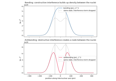
Heitler-London’s insight: bonding vs. antibonding electron density
1927 – 1929 – Kellner and Hylleraas: the Variational Helium Atom#
Heitler and London’s H2 showed that quantum mechanics could explain a bond; helium, the simplest atom with two electrons, was the test of whether it could get an energy right once electron-electron repulsion enters. The repulsion term \(e^2/4\pi\varepsilon_0r_{12}\) makes the Schrodinger equation unsolvable in closed form, so G. W. Kellner (1927) and, far more thoroughly, Egil Hylleraas (1928-1929) turned to the variational principle: any trial wavefunction gives an energy at or above the true ground state, so the best trial function in a family is the one with the lowest energy. The simplest family puts both electrons in hydrogen-like 1s orbitals with an adjustable nuclear charge \(\zeta\), giving
For helium, \(\zeta^*=27/16\): each electron screens 5/16 of the nuclear charge from the other, a first quantitative version of the shielding idea later codified in Slater’s rules. The energy, \(-2.848\,E_h\), lies 2% above the exact nonrelativistic \(-2.9037\,E_h\); Hylleraas closed most of the remaining gap by building the interelectronic distance \(r_{12}\) directly into the trial function, bringing the computed ionization energy into agreement with experiment and putting the variational method, and the idea of electron correlation, at the centre of quantum chemistry.
Implementation: helium_like_variational_energy()
gives \(E(\zeta)\) for any two-electron atom or ion, and
optimize_helium_like_effective_charge()
returns a HeliumVariationalResult with the
optimal screened charge, the variational energy, the first-order
perturbation energy (\(\zeta=Z\)), and the one-electron-removal
energy, which comes out negative for H-: this trial function is too
simple to bind the hydride ion.
References: G. W. Kellner, “Die Ionisierungsspannung des Heliums nach der Schrodingerschen Theorie,” Z. Phys. 44, 91 (1927); E. A. Hylleraas, “Uber den Grundzustand des Heliumatoms,” Z. Phys. 48, 469 (1928); E. A. Hylleraas, “Neue Berechnung der Energie des Heliums im Grundzustande, sowie des tiefsten Terms von Ortho-Helium,” Z. Phys. 54, 347 (1929).
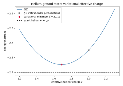
Kellner and Hylleraas: the variational helium atom and its screened charge
1927 – 1932 – Hund and Mulliken’s Molecular-Orbital Theory#
Alongside (and initially at odds with) Heitler and London’s valence-bond picture, Friedrich Hund and Robert Mulliken developed a rival framework built on a different starting assumption: rather than combine two complete atomic wavefunctions and worry about their exchange symmetry directly, first build delocalized one-electron molecular orbitals – typically as a linear combination of atomic orbitals (LCAO), \(\psi=c_A\chi_A+c_B\chi_B\) – spanning the whole molecule, and then fill them with electrons exactly as one fills atomic orbitals, Aufbau and Pauli intact. Hund’s series of papers on molecular spectra and Mulliken’s own long series on diatomic electronic structure worked out the resulting orbital diagrams, bonding/antibonding/nonbonding classification, and correlation to the separated-atom limit in detail; Mulliken’s later synthesis coined “molecular orbital” itself as the field’s now-standard term. Molecular-orbital theory’s LCAO ansatz, rather than valence-bond theory’s atom-centered exchange picture, is what essentially every subsequent computational quantum-chemistry method below – Huckel theory, Hartree-Fock – was built on, less because it is more physically fundamental than valence-bond theory (the two are equivalent at the exact limit) than because its one-electron orbitals reduce so cleanly to a matrix eigenvalue problem.
Implementation: chemistrykit.quantum.systems.hartree_fock.H2PlusVariational
builds exactly this LCAO ansatz for H2+, obtaining the bonding
(\(+\)) and antibonding (\(-\)) combinations directly as the two
eigenvectors of its 2x2 secular equation
(solve()),
with the bonding combination’s energy genuinely lower – the basic
molecular-orbital picture of a covalent bond, obtained here by actual
diagonalization rather than assumed.
References: F. Hund, “Zur Deutung der Molekelspektren,” Z. Phys. 40, 742-764 (1927), and further installments through Z. Phys. 51-63 (1928-1930); R. S. Mulliken, “Electronic States and Band Spectrum Structure in Diatomic Molecules,” Phys. Rev. 32, 186-222 (1928), and “Electronic Structures of Polyatomic Molecules and Valence,” Phys. Rev. 40, 55-62 (1932) (both authors’ molecular-orbital work spans many further papers across this period; the entries cited are representative rather than exhaustive, per standard secondary-literature summaries).
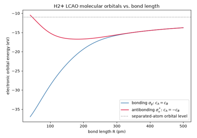
Hund-Mulliken LCAO molecular orbitals of H2+: bonding and antibonding
1929 – Morse’s Anharmonic Potential for Molecular Vibration#
Philip Morse proposed a simple closed-form potential energy curve for a diatomic bond that, unlike the harmonic oscillator’s parabola, actually behaves like a real chemical bond at both extremes: near the equilibrium bond length it is closely parabolic (matching a harmonic oscillator of the same force constant), but at large separation it flattens out to a finite dissociation energy instead of climbing without bound, and at short separation it rises steeply, reflecting nuclear repulsion. Solving the Schrodinger equation for this potential exactly – itself a nontrivial result – gives vibrational energy levels whose spacing shrinks as v increases, unlike the harmonic oscillator’s perfectly even ladder, right up to a highest bound level beyond which the molecule dissociates: the Morse potential remains, a century later, the standard first correction chemists reach for whenever the harmonic approximation to a real bond’s anharmonicity needs to be taken seriously, from infrared overtone intensities to bond-dissociation thermochemistry.
Implementation: chemistrykit.quantum.systems.harmonic_oscillator.MorseOscillator
implements exactly these exact vibrational eigenvalues, with
v_max
giving the highest bound level; compare_harmonic_vs_morse()
tabulates it directly against
QuantumHarmonicOscillator’s
perfectly evenly spaced levels at the same force constant, showing the two
models agree closely near v=0 and diverge sharply as v grows toward
dissociation.
References: P. M. Morse, “Diatomic Molecules According to the Wave Mechanics. II. Vibrational Levels,” Phys. Rev. 34, 57-64 (1929).
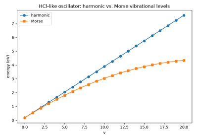
Harmonic vs. Morse vibrational levels: anharmonicity toward dissociation
1931 – Huckel’s pi-Electron Theory and the 4n+2 Aromaticity Rule#
Erich Huckel showed that a conjugated planar pi system’s electronic structure – benzene’s famous, otherwise mysterious extra stability foremost among the puzzles motivating the work – could be captured by an almost brutally simplified molecular-orbital treatment: represent each sp2 carbon’s out-of-plane 2p_z orbital as one atomic-orbital basis function, assume the pi orbitals are mutually orthogonal, and let only directly-bonded neighbors interact at all, via a single shared resonance integral \(\beta\). What survives this drastic simplification is a genuine eigenvalue problem, small enough to solve exactly for real molecules with 1930s hand calculation, and, for a closed ring of n atoms, a strikingly clean electron-counting consequence: a cyclic, planar, fully conjugated system is aromatic – unusually stabilized – only when it holds \(4n+2\) pi electrons for some non-negative integer n, filling every bonding and nonbonding level with no unpaired electron left over in a partially-filled degenerate pair. Benzene’s 6 pi electrons satisfy the rule; cyclobutadiene’s 4 do not, and are correspondingly destabilized (antiaromatic) rather than merely neutral about it.
Implementation: chemistrykit.quantum.systems.huckel.HuckelSystem
builds exactly this Hamiltonian and diagonalizes it via
solve_secular_equation()
with the orthonormal-basis approximation (S=None);
is_aromatic_by_huckel_rule()
checks the \(4n+2\) rule directly against the computed spectrum’s
actual degeneracies (not just electron counting), correctly confirming
benzene aromatic and cyclobutadiene not.
References: E. Huckel, “Quantentheoretische Beitrage zum Benzolproblem. I. Die Elektronenkonfiguration des Benzols und verwandter Verbindungen,” Z. Phys. 70, 204-286 (1931).
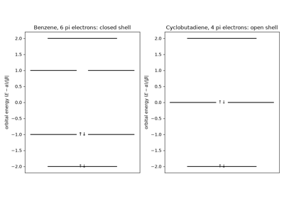
Huckel’s 4n+2 aromaticity rule from the computed pi spectrum
1931 – 1939 – Pauling’s Nature of the Chemical Bond#
Linus Pauling spent the 1930s synthesizing the still-competing valence- bond and molecular-orbital pictures, and quantum mechanics generally, into a working conceptual toolkit chemists without a quantum-mechanics background could actually use: hybridization (mixing an atom’s own s and p orbitals into directional sp, sp2, sp3 combinations to explain observed bond angles and geometries), resonance (describing a molecule, like benzene, whose true electronic structure is not any single Lewis structure but a quantum-mechanical superposition – lower in energy than any one contributing structure alone), and a numerical electronegativity scale built directly from measured bond-dissociation energies. Collected in his 1939 book The Nature of the Chemical Bond, this synthesis – recognized by the 1954 Nobel Prize in Chemistry “for research into the nature of the chemical bond” – did for practicing chemists what Heitler- London and Hund-Mulliken’s original papers, aimed at a physics audience, had not: it made quantum-mechanical bonding concepts into the chemist’s own working vocabulary, “resonance energy” and “hybridization” foremost among them, still in daily use.
Connection: delocalization_energy()
computes exactly what Pauling’s own vocabulary calls a “resonance
energy”: the extra stabilization a delocalized Huckel calculation
predicts relative to the same pi electrons confined to isolated,
localized double bonds – benzene’s negative delocalization energy is a
direct, computed instance of the same resonance-stabilization concept
Pauling made central to 20th-century chemical bonding language.
References: L. Pauling, “The Nature of the Chemical Bond. Application of Results Obtained from the Quantum Mechanics and from a Theory of Paramagnetic Susceptibility to the Structure of Molecules,” J. Am. Chem. Soc. 53, 1367-1400 (1931); L. Pauling, The Nature of the Chemical Bond and the Structure of Molecules and Crystals (Ithaca: Cornell University Press, 1939).
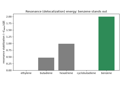
Pauling’s resonance energy as Huckel delocalization energy
1939 – 1953 – Coulson, Frost, and Musulin: Closed-Form Huckel Spectra#
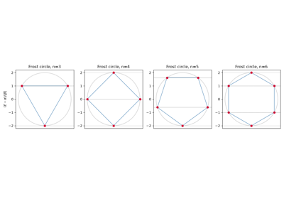
Diagonalizing a Huckel Hamiltonian by hand for anything larger than a handful of atoms was, in the 1930s, a genuine practical obstacle, and two results removed it for the two most chemically important topologies. Charles Coulson found a closed-form trigonometric expression for the eigenvalues of a linear (acyclic) conjugated chain of any length, turning the pi-electron energy of any polyene into a formula rather than a matrix problem. Arthur Frost and Boris Musulin found the analogous closed form for a cyclic ring, and packaged it as a genuinely useful graphical mnemonic still taught today – the “Frost circle”: inscribe a regular n-gon in a circle of radius \(2|\beta|\) point-down, and each vertex’s height directly gives one Huckel eigenvalue, with the degeneracy pattern (a unique lowest level, doubly degenerate pairs above it) visible at a glance.
Implementation: linear_polyene_eigenvalues()
and cyclic_polyene_eigenvalues()
implement exactly these two closed forms, used throughout this
subpackage’s tests and examples as an independent analytic cross-check
of solve()’s
numerical diagonalization – for benzene, reproducing the textbook Frost-
circle pattern \(\alpha+2\beta\), \(\alpha+\beta\) (doubly
degenerate), \(\alpha-\beta\) (doubly degenerate), \(\alpha-2\beta\)
exactly.
References: C. A. Coulson, “The Electronic Structure of Some Polyenes and Aromatic Molecules. VII. Bonds of Fractional Order by the Molecular Orbital Method,” Proc. R. Soc. Lond. A 169, 413-428 (1939); A. A. Frost and B. Musulin, “A Mnemonic Device for Molecular Orbital Energies,” J. Chem. Phys. 21, 572-573 (1953).
1949 – Kuhn’s Free-Electron Model of Conjugated Dyes#
Hans Kuhn proposed treating a linear conjugated dye molecule’s delocalized pi electrons as free particles confined to a one-dimensional box spanning the length of the conjugated chain – ignoring the actual sigma-bond framework, electron-electron repulsion, and everything else a rigorous treatment would need, in exchange for a strikingly simple, essentially parameter-free prediction: as the box (the conjugation length) grows, the particle-in-a-box HOMO-LUMO gap shrinks as \(1/L^2\), red-shifting the predicted absorption – exactly the qualitative trend cyanine dyes and other conjugated chromophores show, and the conceptual basis for tuning a dye’s color by conjugation length that organic and materials chemists still reach for as a first estimate before running anything more expensive.
Implementation: conjugated_dye_absorption_wavelength()
implements exactly this HOMO-LUMO transition-energy formula on top of
ParticleInBox1D,
correctly predicting a cyanine-dye-like chain’s absorption in the visible
range and confirming that adding conjugation (more pi electrons, a longer
box) red-shifts the predicted wavelength, exactly Kuhn’s qualitative
trend.
References: H. Kuhn, “A Quantum-Mechanical Theory of Light Absorption of Organic Dyes and Similar Compounds,” J. Chem. Phys. 17, 1198-1212 (1949).
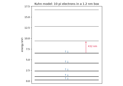
Kuhn’s free-electron model of conjugated dye color
1950 – Boys and the Gaussian-Type Orbital#
Every LCAO calculation above needs, at bottom, actual numbers for overlap, kinetic-energy, and (especially) electron-repulsion integrals between basis functions on different atomic centers – and for the physically natural choice of basis function, an exponentially decaying Slater-type orbital matching the true hydrogen-atom wavefunction’s shape, those multi-center integrals have no closed form at all, and had to be evaluated by slow numerical methods that made anything beyond a diatomic molecule impractical. Samuel Francis Boys’s decisive practical insight was to give up the physically correct exponential shape in exchange for a Gaussian one: unlike two Slater orbitals, the product of two Gaussian functions centered on different atoms is itself just another Gaussian, centered at a third point determined by the two originals – the “Gaussian product theorem” – collapsing every multi-center integral to a one-center problem with a genuine closed form. A single Gaussian approximates a true atomic orbital’s cusp at the nucleus poorly, but combining several of them (a “contracted” Gaussian) recovers useful accuracy while keeping every integral computable in closed form – the foundation essentially every general-purpose quantum-chemistry program since has been built on.
Implementation: chemistrykit.quantum.utils.basis_sets.GaussianPrimitive
implements exactly such a normalized s-type Gaussian primitive, and
overlap_integral(),
kinetic_integral(), and
nuclear_attraction_integral()
give exactly the closed-form Gaussian-product integrals Boys’s method
produces (via boys_f0(), the
zeroth-order Boys function the nuclear-attraction integral reduces to for
s-type functions), used directly by
chemistrykit.quantum.systems.hartree_fock.H2PlusVariational to
build its Hamiltonian and overlap matrices.
electron_repulsion_integral() adds the two-electron integral the
same Gaussian-product theorem makes closed-form, which
RestrictedHartreeFock needs below.
References: S. F. Boys, “Electronic Wave Functions. I. A General Method of Calculation for the Stationary States of Any Molecular System,” Proc. R. Soc. Lond. A 200, 542-554 (1950).
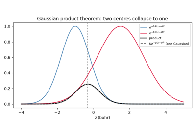
Boys’s Gaussian-type orbitals and the Gaussian product theorem
1951 – Roothaan and Hall’s LCAO Equations#
Clemens Roothaan and, independently and simultaneously, George Hall turned the Hartree-Fock method – until then formulated as an integro- differential equation, practical only for atoms with their exploitable spherical symmetry – into a genuinely computable procedure for molecules of arbitrary shape, by expanding the unknown molecular orbitals in a finite basis (Boys’s Gaussians, above, or any other basis) and showing that the variational condition on the resulting expansion coefficients reduces to a matrix generalized eigenvalue problem, \(HC=SCE\) – the “secular equation” or Roothaan-Hall equation. Because the basis is finite rather than complete, H and S are honest, finite matrices a computer can build and diagonalize directly, and the self-consistent loop this equation sits inside (the Hamiltonian itself depends on the very orbitals being solved for, so the equation is solved repeatedly until the orbitals stop changing) became, and remains, the computational skeleton of essentially every ab initio electronic-structure method built since, Hartree-Fock and its many post-Hartree-Fock and density- functional descendants alike.
Implementation: solve_secular_equation()
implements exactly this generalized eigenvalue problem – via
scipy.linalg.eigh() when a genuine (non-orthogonal) overlap matrix
S is supplied, or the ordinary eigenvalue problem
numpy.linalg.eigh() when the basis is assumed orthonormal (Huckel
theory’s approximation, above) – and is the single shared solver every
variational model in this subpackage
(H2PlusVariational,
HuckelSystem,
RestrictedHartreeFock) reduces to. The
first gallery example builds H and S for the one-electron H2+ from
the Gaussian integrals in chemistrykit.quantum.utils.basis_sets in
bases of growing size and shows the variational energy falling toward
the exact value. For two or more electrons the equation becomes
\(FC=SC\varepsilon\) with a Fock matrix that depends on its own
solution, and RestrictedHartreeFock runs
the full closed-shell self-consistent-field loop. The second example
converges HeH+ to Szabo and Ostlund’s STO-3G energy and traces the RHF
potential curve of H2, including its well-known failure at dissociation.
References: C. C. J. Roothaan, “New Developments in Molecular Orbital Theory,” Rev. Mod. Phys. 23, 69-89 (1951); G. G. Hall, “The Molecular Orbital Theory of Chemical Valency. VIII. A Method of Calculating Ionization Potentials,” Proc. R. Soc. Lond. A 205, 541-552 (1951).
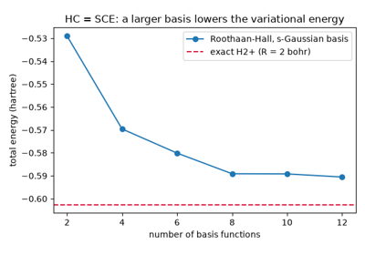
Roothaan-Hall equations: solving HC = SCE in a finite basis
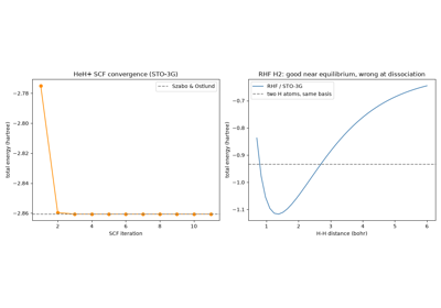
Roothaan-Hall self-consistent field: RHF for HeH+ and H2
1952 – Fukui’s Frontier-Orbital Theory of Reactivity#
Molecular-orbital theory could explain why benzene is stable; Kenichi Fukui, with Teijiro Yonezawa and Haruo Shingu, asked it to predict where a molecule reacts. Their answer was surprisingly economical: of all the occupied orbitals, only the highest one (the HOMO) matters for attack by an electrophile, because its electrons are the most loosely held, and the favoured site is the atom where the HOMO’s density is largest,
(with the LUMO playing the same role for nucleophiles). For naphthalene the Huckel HOMO puts density 0.362 on the alpha carbons and 0.138 on the beta carbons, matching the observed preference for alpha substitution, where total pi-electron densities, all exactly 1 in an alternant hydrocarbon, predict nothing. Extended to pericyclic reactions and to the interaction of one molecule’s HOMO with another’s LUMO, frontier orbital theory earned Fukui a share of the 1981 Nobel Prize in Chemistry with Roald Hoffmann.
Implementation: frontier_electron_density()
returns \(f_r\) for the HOMO or LUMO of any
HuckelSystem, refusing
cases where the frontier orbital is degenerate (benzene) and the density
is not uniquely defined.
References: K. Fukui, T. Yonezawa, and H. Shingu, “A Molecular Orbital Theory of Reactivity in Aromatic Hydrocarbons,” J. Chem. Phys. 20, 722-725 (1952).
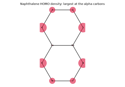
Fukui’s frontier orbitals: why naphthalene reacts at the alpha position
1969 – Hehre, Stewart, and Pople’s STO-nG Minimal Basis#
Boys’s Gaussians made molecular integrals computable but had the wrong shape. Slater orbitals had the right shape but intractable integrals. Warren Hehre, Robert Stewart and John Pople resolved the trade-off pragmatically. They fitted each Slater orbital, once and for all, by a fixed least-squares combination of \(n\) Gaussians (“STO-nG”). Since the Slater exponent only rescales the function, one table of \(\zeta=1\) expansion coefficients serves every element: the Gaussian exponents simply scale as \(\zeta^2\). STO-3G, three Gaussians per orbital, was the default basis of Pople’s GAUSSIAN 70 program, the first widely distributed ab initio code. It put Hartree-Fock calculations on real molecules within reach of ordinary chemists, part of the work recognized by Pople’s 1998 Nobel Prize.
Implementation: sto3g_1s()
builds the contracted STO-3G 1s function
(ContractedGaussian) for
any \(\zeta\), and RestrictedHartreeFock
uses it for its H2 and HeH+ presets. The example compares the
contraction with its Slater target and a single Gaussian, then
reproduces Szabo and Ostlund’s STO-3G energies for both molecules.
References: W. J. Hehre, R. F. Stewart, and J. A. Pople, “Self-Consistent Molecular-Orbital Methods. I. Use of Gaussian Expansions of Slater-Type Atomic Orbitals,” J. Chem. Phys. 51, 2657-2664 (1969).
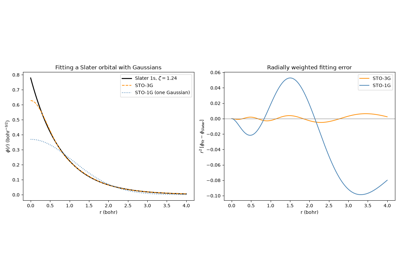
Hehre, Stewart and Pople’s STO-3G basis: three Gaussians for one Slater orbital