Heitler-London’s insight: bonding vs. antibonding electron density

Walter Heitler and Fritz London’s 1927 quantum-mechanical treatment of H2 – the paper usually credited with founding quantum chemistry as a field – showed for the first time why two hydrogen atoms bind: the symmetric (in-phase) combination of their two atomic orbitals builds up electron density in the region between the nuclei, lowering the energy below that of the separated atoms, while the antisymmetric (out-of-phase) combination depletes density there and raises the energy instead. Their original calculation used two-electron integrals this package does not implement (chemistrykit.quantum.utils.basis_sets stops at the one-electron integrals H2PlusVariational needs for H2+), but the same qualitative physics – constructive vs. destructive interference of atomic orbitals along the bond axis – is exactly what H2+’s own bonding and antibonding molecular orbitals show, using the genuine LCAO coefficients solve() computes, not an assumed equal-weight combination.

import matplotlib.pyplot as plt
import numpy as np

from chemistrykit.quantum.systems.hartree_fock import H2PlusVariational

BOND_LENGTH = 106.0e-12  # H2+'s experimental equilibrium bond length
BOHR_RADIUS = 5.29177e-11

h2plus = H2PlusVariational(bond_length=BOND_LENGTH)
optimization = h2plus.optimize_exponent(alpha_guess=1.0 / BOHR_RADIUS**2)
result = h2plus.solve(optimization.optimized_alpha)
print(f"Optimized exponent alpha = {optimization.optimized_alpha:.4e} m^-2")
print(f"Bonding coefficients     (c_A, c_B) = {result.orbital_coefficients(0)}")
print(f"Antibonding coefficients (c_A, c_B) = {result.orbital_coefficients(1)}")

Optimized exponent alpha = 1.5553e+20 m^-2
Bonding coefficients     (c_A, c_B) = [-0.59394159 -0.59394159]
Antibonding coefficients (c_A, c_B) = [ 0.92637692 -0.92637692]

Evaluate each normalized s-Gaussian along the internuclear (z) axis directly, then form the two LCAO combinations with the actual computed coefficients:

def gaussian_along_axis(alpha, center_z, z):
    normalization = (2.0 * alpha / np.pi) ** 0.75
    return normalization * np.exp(-alpha * (z - center_z) ** 2)


z = np.linspace(-3.0 * BOND_LENGTH, 3.0 * BOND_LENGTH, 801)
chi_a = gaussian_along_axis(optimization.optimized_alpha, -BOND_LENGTH / 2.0, z)
chi_b = gaussian_along_axis(optimization.optimized_alpha, BOND_LENGTH / 2.0, z)

c_a_bond, c_b_bond = result.orbital_coefficients(0)
c_a_anti, c_b_anti = result.orbital_coefficients(1)
psi_bonding = c_a_bond * chi_a + c_b_bond * chi_b
psi_antibonding = c_a_anti * chi_a + c_b_anti * chi_b

# The "no interference" reference for each state drops just its own cross
# (interference) term, |c_a*chi_a + c_b*chi_b|^2 -> c_a^2*chi_a^2 +
# c_b^2*chi_b^2, holding that state's own LCAO normalization fixed -- the
# fair baseline for isolating what constructive/destructive interference
# alone contributes, since the bonding and antibonding states are
# normalized to different overall magnitudes (S_AB shifts the bonding
# normalization down and the antibonding normalization up).
no_interference_bond = c_a_bond**2 * chi_a**2 + c_b_bond**2 * chi_b**2
no_interference_anti = c_a_anti**2 * chi_a**2 + c_b_anti**2 * chi_b**2

fig, (ax1, ax2) = plt.subplots(2, 1, figsize=(7, 7), sharex=True)
ax1.plot(z * 1.0e12, psi_bonding**2, color="steelblue", label="bonding |psi_+|^2")
ax1.plot(z * 1.0e12, no_interference_bond, color="gray", linestyle=":", label="same state, interference term dropped")
ax1.axvline(-BOND_LENGTH / 2.0 * 1.0e12, color="black", linestyle="--", linewidth=0.6)
ax1.axvline(BOND_LENGTH / 2.0 * 1.0e12, color="black", linestyle="--", linewidth=0.6)
ax1.set_ylabel(r"$|\psi_+|^2$")
ax1.set_title("Bonding: constructive interference builds up density between the nuclei")
ax1.legend()

ax2.plot(z * 1.0e12, psi_antibonding**2, color="crimson", label="antibonding |psi_-|^2")
ax2.plot(z * 1.0e12, no_interference_anti, color="gray", linestyle=":", label="same state, interference term dropped")
ax2.axvline(-BOND_LENGTH / 2.0 * 1.0e12, color="black", linestyle="--", linewidth=0.6)
ax2.axvline(BOND_LENGTH / 2.0 * 1.0e12, color="black", linestyle="--", linewidth=0.6)
ax2.set_xlabel("position along internuclear axis (pm)")
ax2.set_ylabel(r"$|\psi_-|^2$")
ax2.set_title("Antibonding: destructive interference creates a node between the nuclei")
ax2.legend()
fig.tight_layout()

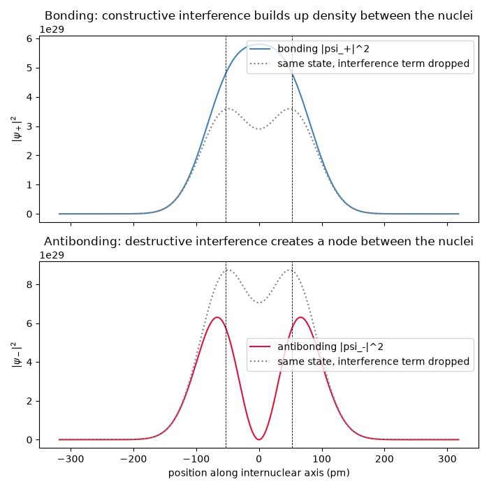
Directly at the midpoint between the two nuclei, the interference term genuinely adds density for the bonding state (above its own no-interference baseline) and genuinely removes it for the antibonding state (down to essentially a node) – exactly the mechanism Heitler and London identified:

midpoint_index = len(z) // 2
bonding_enhancement = psi_bonding[midpoint_index] ** 2 - no_interference_bond[midpoint_index]
antibonding_depletion = psi_antibonding[midpoint_index] ** 2 - no_interference_anti[midpoint_index]
print(f"\nAt the midpoint: bonding density         = {psi_bonding[midpoint_index] ** 2:.4e} (interference contributes {bonding_enhancement:+.4e})")
print(f"                 antibonding density     = {psi_antibonding[midpoint_index] ** 2:.4e} (interference contributes {antibonding_depletion:+.4e})")

plt.show()

At the midpoint: bonding density         = 5.8026e+29 (interference contributes +2.9013e+29)
                 antibonding density     = 1.5625e-02 (interference contributes -7.0580e+29)