Hund-Mulliken LCAO molecular orbitals of H2+: bonding and antibonding

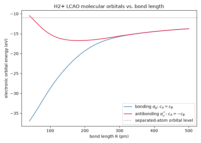
Hund and Mulliken’s molecular-orbital theory builds one-electron orbitals spread over the whole molecule as a linear combination of atomic orbitals, \(\psi_\pm=c_A\chi_A\pm c_B\chi_B\). H2PlusVariational does this for H2+ with one Gaussian orbital per proton: diagonalizing the 2x2 problem gives the in-phase bonding orbital (equal coefficients, energy below the isolated-atom level) and the out-of-phase antibonding orbital (opposite coefficients, energy above it). Following both orbital energies from short bond lengths out to separated atoms gives Mulliken’s correlation diagram for the simplest molecule.

import matplotlib.pyplot as plt
import numpy as np

from chemistrykit.constants import ELECTRONVOLT
from chemistrykit.quantum.systems.hartree_fock import H2PlusVariational

BOHR_RADIUS = 5.29177e-11
h2plus = H2PlusVariational(bond_length=106.0e-12)
alpha = h2plus.optimize_exponent(1.0 / BOHR_RADIUS**2).optimized_alpha
result = h2plus.solve(alpha)
for i, name in enumerate(("bonding", "antibonding")):
    c_a, c_b = result.orbital_coefficients(i)
    print(f"{name:12s} E = {result.energies[i] / ELECTRONVOLT:8.3f} eV   (c_A, c_B) = ({c_a:+.4f}, {c_b:+.4f})")

bonding      E =  -28.018 eV   (c_A, c_B) = (-0.5939, -0.5939)
antibonding  E =  -15.437 eV   (c_A, c_B) = (+0.9264, -0.9264)

Orbital energies as a function of bond length, at a fixed exponent so the separated-atom limit is a single atomic level. The bonding MO drops below that level as the atoms approach; the antibonding MO rises above it, and rises further than the bonding MO falls because of the overlap S_AB.

R_pm = np.linspace(40.0, 500.0, 80)
bonding, antibonding, overlap = [], [], []
for R in R_pm:
    res = H2PlusVariational(bond_length=R * 1.0e-12).solve(alpha)
    bonding.append(res.energies[0] / ELECTRONVOLT)
    antibonding.append(res.energies[1] / ELECTRONVOLT)
    overlap.append(res.overlap[0, 1])
atom_level = H2PlusVariational(bond_length=1.0e-8).solve(alpha).energies[0] / ELECTRONVOLT

fig, ax = plt.subplots(figsize=(7, 5))
ax.plot(R_pm, bonding, color="steelblue", label=r"bonding $\sigma_g$: $c_A=c_B$")
ax.plot(R_pm, antibonding, color="crimson", label=r"antibonding $\sigma_u^*$: $c_A=-c_B$")
ax.axhline(atom_level, color="gray", linestyle=":", label="separated-atom orbital level")
ax.set_xlabel("bond length R (pm)")
ax.set_ylabel("electronic orbital energy (eV)")
ax.set_title("H2+ LCAO molecular orbitals vs. bond length")
ax.legend()
fig.tight_layout()

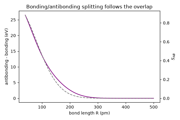
The splitting is driven by the atomic-orbital overlap: both vanish together as the atoms separate.

fig2, ax2 = plt.subplots(figsize=(6, 4))
ax2.plot(R_pm, np.array(antibonding) - np.array(bonding), color="purple", label="MO splitting (eV)")
ax2.set_xlabel("bond length R (pm)")
ax2.set_ylabel("antibonding - bonding (eV)")
ax3 = ax2.twinx()
ax3.plot(R_pm, overlap, color="gray", linestyle="--", label=r"overlap $S_{AB}$")
ax3.set_ylabel(r"$S_{AB}$")
ax2.set_title("Bonding/antibonding splitting follows the overlap")
fig2.tight_layout()

plt.show()