Born-Oppenheimer clamped-nuclei potential curve of H2+

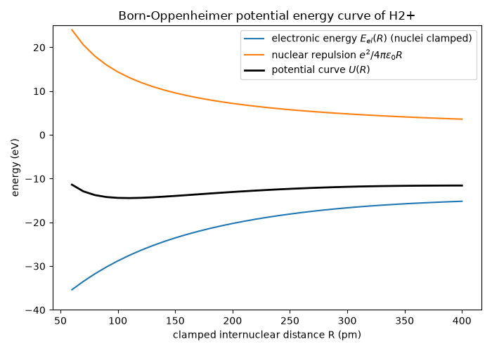
Born and Oppenheimer separated the fast electrons from the slow nuclei: first solve the electronic problem with the nuclei clamped at a fixed separation R, then let the nuclei move on the resulting potential energy curve \(U(R)=E_{el}(R)+e^2/4\pi\varepsilon_0R\). Here each point of the curve is a separate clamped-nuclei calculation with H2PlusVariational (bond_length is a fixed input, never a dynamical variable). The curvature at the minimum then gives a nuclear vibrational frequency, and because the electronic curve does not depend on nuclear mass, H2+ and D2+ share the same curve but have different zero-point energies.

import matplotlib.pyplot as plt
import numpy as np

from chemistrykit.constants import ATOMIC_MASS_UNIT, ELECTRONVOLT, HBAR, PROTON_MASS
from chemistrykit.quantum.systems.hartree_fock import H2PlusVariational

BOHR_RADIUS = 5.29177e-11
R = np.linspace(60.0, 400.0, 35) * 1.0e-12
electronic, repulsion, total = [], [], []
for Ri in R:
    system = H2PlusVariational(bond_length=Ri)
    opt = system.optimize_exponent(1.0 / BOHR_RADIUS**2)
    total.append(opt.optimized_energy)
    repulsion.append(system.nuclear_repulsion)
    electronic.append(opt.optimized_energy - system.nuclear_repulsion)
electronic, repulsion, total = (np.array(a) / ELECTRONVOLT for a in (electronic, repulsion, total))

fig, ax = plt.subplots(figsize=(7, 5))
ax.plot(R * 1e12, electronic, label=r"electronic energy $E_{el}(R)$ (nuclei clamped)")
ax.plot(R * 1e12, repulsion, label=r"nuclear repulsion $e^2/4\pi\varepsilon_0 R$")
ax.plot(R * 1e12, total, color="black", linewidth=2, label=r"potential curve $U(R)$")
ax.set_ylim(-40, 25)
ax.set_xlabel("clamped internuclear distance R (pm)")
ax.set_ylabel("energy (eV)")
ax.set_title("Born-Oppenheimer potential energy curve of H2+")
ax.legend()
fig.tight_layout()

Fit a parabola to U(R) near its minimum for the force constant, then solve the nuclear problem (harmonic approximation) for two isotopologues.

i_min = int(np.argmin(total))
window = slice(max(i_min - 3, 0), i_min + 4)
coeffs = np.polyfit(R[window], total[window] * ELECTRONVOLT, 2)
R_e = -coeffs[1] / (2.0 * coeffs[0])
k = 2.0 * coeffs[0]
print(f"Equilibrium R_e = {R_e * 1e12:.1f} pm, force constant k = {k:.0f} N/m")

deuteron_mass = 2.01355321 * ATOMIC_MASS_UNIT
for name, mu in (("H2+", PROTON_MASS / 2.0), ("D2+", deuteron_mass / 2.0)):
    omega = np.sqrt(k / mu)
    zpe = 0.5 * HBAR * omega / ELECTRONVOLT
    print(f"{name}: same U(R); harmonic zero-point energy = {zpe * 1000:.0f} meV")

x = np.linspace(R[0], R[-1], 300)
fig2, ax2 = plt.subplots(figsize=(6, 4))
ax2.plot(R * 1e12, total, "o", color="black", label="clamped-nuclei points")
ax2.plot(x * 1e12, np.polyval(coeffs, x) / ELECTRONVOLT, color="gray", linestyle="--", label="harmonic fit near $R_e$")
for mu, color, name in ((PROTON_MASS / 2.0, "steelblue", "H2+"), (deuteron_mass / 2.0, "crimson", "D2+")):
    level = np.polyval(coeffs, R_e) / ELECTRONVOLT + 0.5 * HBAR * np.sqrt(k / mu) / ELECTRONVOLT
    ax2.axhline(level, color=color, linewidth=1, label=f"{name} v=0 level")
ax2.set_xlim(60, 250)
ax2.set_ylim(total[i_min] - 0.5, total[i_min] + 2.0)
ax2.set_xlabel("R (pm)")
ax2.set_ylabel("energy (eV)")
ax2.set_title("One electronic curve, isotope-dependent nuclear levels")
ax2.legend(fontsize=8)
fig2.tight_layout()

plt.show()

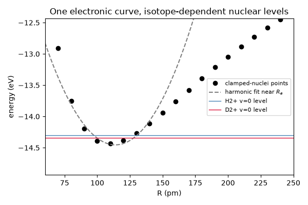
Equilibrium R_e = 113.8 pm, force constant k = 180 N/m
H2+: same U(R); harmonic zero-point energy = 153 meV
D2+: same U(R); harmonic zero-point energy = 108 meV