Boys’s Gaussian-type orbitals and the Gaussian product theorem

S. F. Boys (1950) proposed building molecular wavefunctions from Gaussian functions \(e^{-\alpha r^2}\) instead of the physically natural Slater-type \(e^{-\zeta r}\). The payoff is the Gaussian product theorem: the product of two Gaussians on different centres is a single Gaussian on a point between them, so every multi-centre integral reduces to a closed form. 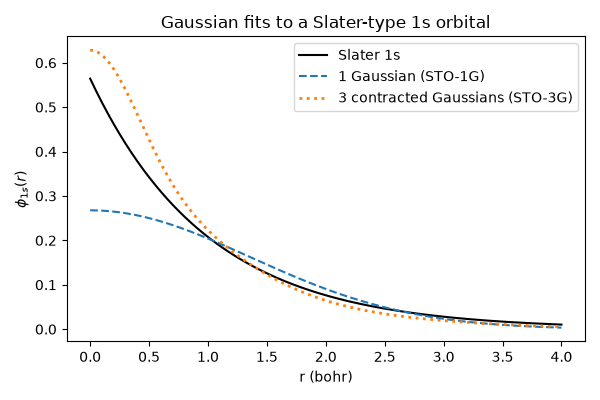This example checks the theorem numerically, checks the closed-form overlap integral (overlap_integral()) and the Boys function (boys_f0()) against brute-force quadrature, and shows the price paid: one Gaussian has no cusp at the nucleus, while a contraction of three (STO-3G) comes close to the Slater 1s orbital.

import matplotlib.pyplot as plt
import numpy as np
from scipy.integrate import quad

from chemistrykit.quantum.utils.basis_sets import GaussianPrimitive, boys_f0, overlap_integral

# Work in bohr (a0 = 1) for readability; the integrals are scale-free here.
a, b = 0.8, 0.3  # exponents
A, B = -1.0, 1.5  # centres on the z axis
p = a + b
P = (a * A + b * B) / p
K = np.exp(-a * b / p * (A - B) ** 2)

z = np.linspace(-4.0, 5.0, 600)
product = np.exp(-a * (z - A) ** 2) * np.exp(-b * (z - B) ** 2)
single = K * np.exp(-p * (z - P) ** 2)
print(f"Gaussian product theorem: centre P = {P:.4f}, max |difference| = {np.max(np.abs(product - single)):.1e}")

fig, ax = plt.subplots(figsize=(7, 4))
ax.plot(z, np.exp(-a * (z - A) ** 2), color="steelblue", label=rf"$e^{{-{a}(z-A)^2}}$")
ax.plot(z, np.exp(-b * (z - B) ** 2), color="crimson", label=rf"$e^{{-{b}(z-B)^2}}$")
ax.plot(z, product, color="black", linewidth=3, alpha=0.4, label="product")
ax.plot(z, single, color="black", linestyle="--", label=r"$K e^{-p(z-P)^2}$ (one Gaussian)")
ax.axvline(P, color="gray", linestyle=":")
ax.set_xlabel("z (bohr)")
ax.set_title("Gaussian product theorem: two centres collapse to one")
ax.legend(fontsize=8)
fig.tight_layout()

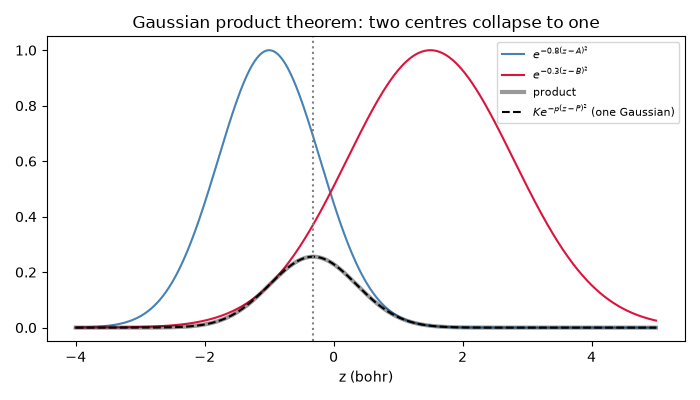
Gaussian product theorem: centre P = -0.3182, max |difference| = 1.1e-16

The closed-form two-centre overlap against a direct 3D grid sum.

ga = GaussianPrimitive(a, [0.0, 0.0, A])
gb = GaussianPrimitive(b, [0.0, 0.0, B])
h = 0.08
grid = np.arange(-7.0, 7.0 + h, h)
X, Y = np.meshgrid(grid, grid, indexing="ij")
numeric = 0.0
for zk in grid:
    r2a = X**2 + Y**2 + (zk - A) ** 2
    r2b = X**2 + Y**2 + (zk - B) ** 2
    numeric += np.sum(ga.normalization * np.exp(-a * r2a) * gb.normalization * np.exp(-b * r2b)) * h**3
print(f"overlap: closed form = {overlap_integral(ga, gb):.6f}, grid sum = {numeric:.6f}")

for x in (0.0, 0.5, 2.0, 10.0):
    direct, _ = quad(lambda t, x=x: np.exp(-x * t**2), 0.0, 1.0)
    print(f"Boys F0({x:4.1f}): closed form = {boys_f0(x):.8f}, quadrature = {direct:.8f}")

overlap: closed form = 0.214978, grid sum = 0.214978
Boys F0( 0.0): closed form = 1.00000000, quadrature = 1.00000000
Boys F0( 0.5): closed form = 0.85562439, quadrature = 0.85562439
Boys F0( 2.0): closed form = 0.59814401, quadrature = 0.59814401
Boys F0(10.0): closed form = 0.28024739, quadrature = 0.28024739

The cost: a Gaussian is flat at the nucleus where the Slater 1s orbital has a cusp. Contracting three Gaussians (the STO-3G fit to a zeta = 1 Slater orbital, Hehre, Stewart & Pople 1969) repairs most of the shape.

r = np.linspace(0.0, 4.0, 400)
slater = np.exp(-r) / np.sqrt(np.pi)


def contracted(exponents, coefficients):
    return sum(c * (2.0 * e / np.pi) ** 0.75 * np.exp(-e * r**2) for e, c in zip(exponents, coefficients))


sto1g = contracted([0.270950], [1.0])
sto3g = contracted([3.42525091, 0.62391373, 0.16885540], [0.15432897, 0.53532814, 0.44463454])
fig2, ax2 = plt.subplots(figsize=(6, 4))
ax2.plot(r, slater, color="black", label="Slater 1s")
ax2.plot(r, sto1g, "--", label="1 Gaussian (STO-1G)")
ax2.plot(r, sto3g, ":", linewidth=2, label="3 contracted Gaussians (STO-3G)")
ax2.set_xlabel("r (bohr)")
ax2.set_ylabel(r"$\phi_{1s}(r)$")
ax2.set_title("Gaussian fits to a Slater-type 1s orbital")
ax2.legend()
fig2.tight_layout()

plt.show()