Roothaan-Hall equations: solving HC = SCE in a finite basis

Roothaan and Hall turned the molecular orbital problem into matrix algebra: expand each orbital in a finite, non-orthogonal basis and the variational condition becomes the generalized eigenvalue problem \(HC=SCE\), solved here by solve_secular_equation(). For the one-electron H2+ the Fock matrix is just the core Hamiltonian, so the equation is solved exactly once in each basis. The example shows that the overlap matrix S matters, that Lowdin’s symmetric orthogonalization \(S^{-1/2}HS^{-1/2}\) gives the same answer, and that enlarging the basis lowers the energy toward the exact H2+ value, as the variational principle requires.

import matplotlib.pyplot as plt
import numpy as np
from scipy.linalg import fractional_matrix_power

from chemistrykit.constants import ELEMENTARY_CHARGE, VACUUM_PERMITTIVITY
from chemistrykit.quantum.systems.helium import HARTREE_ENERGY
from chemistrykit.quantum.utils.basis_sets import GaussianPrimitive, kinetic_integral, nuclear_attraction_integral, overlap_integral
from chemistrykit.quantum.utils.secular_equation import solve_secular_equation

A0 = 5.29177210903e-11
R = 2.0 * A0  # H2+ near its equilibrium bond length, 2 bohr
centres = [np.array([0.0, 0.0, -R / 2]), np.array([0.0, 0.0, R / 2])]
nuclear_repulsion = ELEMENTARY_CHARGE**2 / (4.0 * np.pi * VACUUM_PERMITTIVITY * R)


def build_matrices(exponents_bohr):
    """Core Hamiltonian H and overlap S for s-Gaussians with the given exponents on both protons."""
    basis = [GaussianPrimitive(e / A0**2, c) for c in centres for e in exponents_bohr]
    n = len(basis)
    H, S = np.empty((n, n)), np.empty((n, n))
    for i, gi in enumerate(basis):
        for j, gj in enumerate(basis):
            S[i, j] = overlap_integral(gi, gj)
            H[i, j] = kinetic_integral(gi, gj) + sum(nuclear_attraction_integral(gi, gj, 1.0, c) for c in centres)
    return H, S


H, S = build_matrices([0.4166])
E_with_S, C = solve_secular_equation(H, S)
E_without_S = np.linalg.eigvalsh(H)
Sm12 = np.real(fractional_matrix_power(S, -0.5))
E_lowdin = np.linalg.eigvalsh(Sm12 @ H @ Sm12)
print(f"S =\n{np.round(S, 4)}")
print(f"HC=SCE eigenvalues (hartree):          {E_with_S / HARTREE_ENERGY}")
print(f"Lowdin S^-1/2 H S^-1/2 eigenvalues:    {E_lowdin / HARTREE_ENERGY}")
print(f"ignoring S (HC=CE) eigenvalues:        {E_without_S / HARTREE_ENERGY}")
print(f"C^T S C = I? {np.allclose(C.T @ S @ C, np.eye(2))}")

S =
[[1.     0.4347]
 [0.4347 1.    ]]
HC=SCE eigenvalues (hartree):          [-1.03000811 -0.57067504]
Lowdin S^-1/2 H S^-1/2 eigenvalues:    [-1.03000811 -0.57067504]
ignoring S (HC=CE) eigenvalues:        [-1.47770748 -0.32262762]
C^T S C = I? True

Enlarging the basis: nested sets of s-Gaussian exponents on each proton. Each larger basis contains the smaller one, so the variational energy can only go down; it approaches the exact H2+ energy at R = 2 bohr, -0.6026 hartree (total, including nuclear repulsion). A pure s basis cannot polarize along the bond, so it stops a little short.

exponent_pool = [0.4, 1.6, 0.1, 6.4, 0.025, 25.6]
sizes = range(1, len(exponent_pool) + 1)
energies = []
for n in sizes:
    Hn, Sn = build_matrices(exponent_pool[:n])
    En, _ = solve_secular_equation(Hn, Sn)
    energies.append((En[0] + nuclear_repulsion) / HARTREE_ENERGY)
    print(f"{2 * n:2d} basis functions: total energy = {energies[-1]:.5f} hartree")

fig, ax = plt.subplots(figsize=(6, 4))
ax.plot([2 * n for n in sizes], energies, "o-", label="Roothaan-Hall, s-Gaussian basis")
ax.axhline(-0.6026, color="crimson", linestyle="--", label="exact H2+ (R = 2 bohr)")
ax.set_xlabel("number of basis functions")
ax.set_ylabel("total energy (hartree)")
ax.set_title("HC = SCE: a larger basis lowers the variational energy")
ax.legend()
fig.tight_layout()

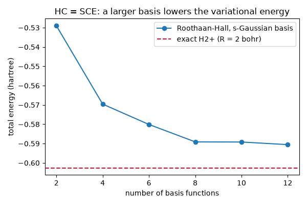
 2 basis functions: total energy = -0.52900 hartree
 4 basis functions: total energy = -0.56958 hartree
 6 basis functions: total energy = -0.58011 hartree
 8 basis functions: total energy = -0.58912 hartree
10 basis functions: total energy = -0.58920 hartree
12 basis functions: total energy = -0.59055 hartree

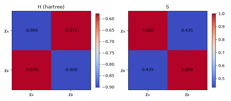
The matrices themselves for the smallest basis: the off-diagonal overlap is what turns the ordinary eigenproblem into a generalized one.

fig2, (ax1, ax2) = plt.subplots(1, 2, figsize=(8, 3.5))
for axis, M, title in ((ax1, H / HARTREE_ENERGY, "H (hartree)"), (ax2, S, "S")):
    im = axis.imshow(M, cmap="coolwarm")
    for (i, j), v in np.ndenumerate(M):
        axis.text(j, i, f"{v:.3f}", ha="center", va="center")
    axis.set_xticks([0, 1], ["$\\chi_A$", "$\\chi_B$"])
    axis.set_yticks([0, 1], ["$\\chi_A$", "$\\chi_B$"])
    axis.set_title(title)
    fig2.colorbar(im, ax=axis, shrink=0.8)
fig2.tight_layout()

plt.show()