Lewis’s shared electron pair: two opposite-spin electrons in one bonding orbital

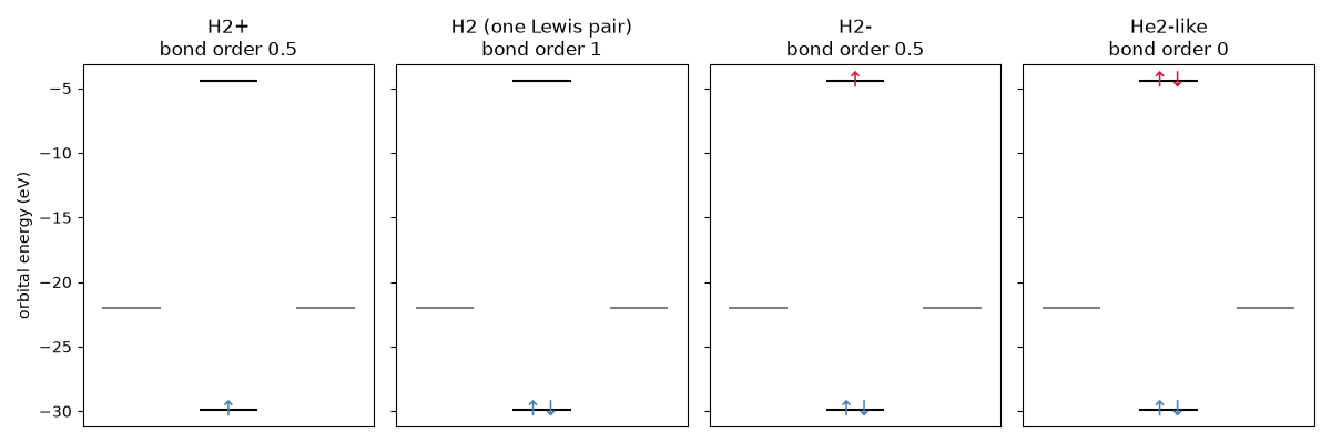
G. N. Lewis’s 1916 covalent bond is a pair of electrons shared between two atoms. In molecular-orbital language that pair is two electrons of opposite spin in the same bonding orbital. Using the two orbitals of a hydrogen-like diatomic from H2PlusVariational (at the H2 bond length, electron-electron repulsion neglected), fill them with 1 to 4 electrons: the bond order \((n_{bonding}-n_{antibonding})/2\) is 1 exactly when a single Lewis pair sits in the bonding orbital, and adding a second pair to the antibonding orbital cancels the bond (the He2 case).

import matplotlib.pyplot as plt
import numpy as np

from chemistrykit.constants import ELECTRONVOLT
from chemistrykit.quantum.systems.hartree_fock import H2PlusVariational

BOHR_RADIUS = 5.29177e-11
ALPHA = 1.0 / BOHR_RADIUS**2
diatomic = H2PlusVariational(bond_length=74.0e-12)
e_bond, e_anti = diatomic.solve(ALPHA).energies / ELECTRONVOLT
# Reference: an electron left in one atomic orbital at the same geometry, H_AA.
e_atom = diatomic.hamiltonian(ALPHA)[0, 0] / ELECTRONVOLT
print(f"atomic-orbital level H_AA {e_atom:.2f} eV, bonding MO {e_bond:.2f} eV, antibonding MO {e_anti:.2f} eV")

cases = [("H2+", 1), ("H2 (one Lewis pair)", 2), ("H2-", 3), ("He2-like", 4)]
occupations = {1: (1, 0), 2: (2, 0), 3: (2, 1), 4: (2, 2)}

atomic-orbital level H_AA -21.96 eV, bonding MO -29.91 eV, antibonding MO -4.45 eV

Orbital diagrams: arrows are electrons, paired arrows are Lewis’s shared pair.

fig, axes = plt.subplots(1, 4, figsize=(12, 4), sharey=True)
for ax, (name, n) in zip(axes, cases):
    n_b, n_a = occupations[n]
    for x in (-1.0, 1.0):
        ax.hlines(e_atom, x - 0.3, x + 0.3, color="gray")
    ax.hlines([e_bond, e_anti], -0.3, 0.3, color="black")
    arrows = {1: "↑", 2: "↑↓"}
    if n_b:
        ax.text(0.0, e_bond, arrows[n_b], ha="center", va="center", fontsize=14, color="steelblue")
    if n_a:
        ax.text(0.0, e_anti, arrows[n_a], ha="center", va="center", fontsize=14, color="crimson")
    ax.set_xlim(-1.5, 1.5)
    ax.set_xticks([])
    ax.set_title(f"{name}\nbond order {(n_b - n_a) / 2:g}")
axes[0].set_ylabel("orbital energy (eV)")
fig.tight_layout()

Sum of orbital energies relative to the unshared atomic-orbital level \(H_{AA}\): the second electron in the bonding orbital doubles the stabilization (the pair bond), while antibonding electrons, raised more than bonding ones are lowered, undo it and more.

n_electrons = np.array([n for _, n in cases])
bond_order = np.array([(occupations[n][0] - occupations[n][1]) / 2 for n in n_electrons])
energy_change = np.array([occupations[n][0] * e_bond + occupations[n][1] * e_anti - n * e_atom for n in n_electrons])
for (name, _), bo, de in zip(cases, bond_order, energy_change):
    print(f"{name:20s} bond order {bo:3.1f}  orbital-energy change {de:+7.2f} eV")

fig2, ax2 = plt.subplots(figsize=(6, 4))
ax2.bar(n_electrons - 0.2, bond_order, width=0.4, color="steelblue", label="bond order")
ax3 = ax2.twinx()
ax3.bar(n_electrons + 0.2, energy_change, width=0.4, color="darkorange", label="orbital-energy change (eV)")
ax2.set_xticks(n_electrons, [name for name, _ in cases], fontsize=8)
ax2.set_ylabel("bond order")
ax3.set_ylabel(r"$\sum n_i\varepsilon_i - N H_{AA}$ (eV)")
ax2.set_title("The shared pair: bond order peaks at two electrons")
fig2.tight_layout()

plt.show()

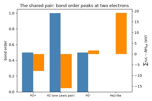
H2+                  bond order 0.5  orbital-energy change   -7.94 eV
H2 (one Lewis pair)  bond order 1.0  orbital-energy change  -15.88 eV
H2-                  bond order 0.5  orbital-energy change   +1.64 eV
He2-like             bond order 0.0  orbital-energy change  +19.15 eV