Dennison’s rigid rotor: rotational levels and the microwave spectrum

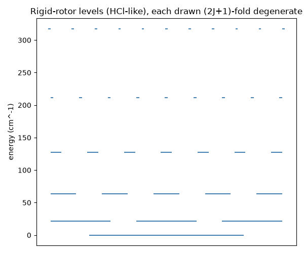
Dennison (1926) solved Schrodinger’s equation for a rotating diatomic molecule, giving levels \(E_J=J(J+1)\hbar^2/2I\). Builds an HCl-like RigidRotor from its atomic masses and bond length (from_diatomic()), plots its energy-level diagram (each level’s height showing its \((2J+1)\)-fold degeneracy), and shows that the \(J\to J+1\) microwave absorption lines are evenly spaced by \(2B\).

import matplotlib.pyplot as plt
import numpy as np
import scipy.constants as sc

from chemistrykit.quantum.systems.rigid_rotor import RigidRotor
from chemistrykit.quantum.visualizers.quantum_plots import plot_energy_levels

rotor = RigidRotor.from_diatomic(mass1=1.008 * sc.atomic_mass, mass2=34.97 * sc.atomic_mass, bond_length=127.5e-12)
print(f"Moment of inertia I = {rotor.moment_of_inertia:.4e} kg m^2")
print(f"Rotational constant B = {rotor.rotational_constant / sc.h / sc.c / 100.0:.4f} cm^-1")

J_values = np.arange(0, 6)
energies_cm1 = np.array([rotor.energy(J) for J in J_values]) / sc.h / sc.c / 100.0
for J, e in zip(J_values, energies_cm1, strict=True):
    print(f"J={J}: E={e:.3f} cm^-1, degeneracy={rotor.degeneracy(J)}")

Moment of inertia I = 2.6448e-47 kg m^2
Rotational constant B = 10.5842 cm^-1
J=0: E=0.000 cm^-1, degeneracy=1
J=1: E=21.168 cm^-1, degeneracy=3
J=2: E=63.505 cm^-1, degeneracy=5
J=3: E=127.010 cm^-1, degeneracy=7
J=4: E=211.683 cm^-1, degeneracy=9
J=5: E=317.525 cm^-1, degeneracy=11

Each level is genuinely (2J+1)-fold degenerate – drawn here as that many short segments at the same height:

all_energies_with_degeneracy = np.concatenate([np.full(rotor.degeneracy(J), rotor.energy(J)) for J in J_values]) / sc.h / sc.c / 100.0

fig, ax = plt.subplots(figsize=(6, 5))
plot_energy_levels(all_energies_with_degeneracy, ax=ax, color="steelblue")
ax.set_ylabel("energy (cm^-1)")
ax.set_title("Rigid-rotor levels (HCl-like), each drawn (2J+1)-fold degenerate")
fig.tight_layout()

The J -> J+1 absorption transitions are evenly spaced by 2B – the defining signature of a rigid-rotor rotational spectrum:

transition_J = np.arange(0, 5)
transition_energies_cm1 = np.array([rotor.transition_energy(J) for J in transition_J]) / sc.h / sc.c / 100.0
spacings = np.diff(transition_energies_cm1)
print(f"Transition spacings (should all equal 2B): {spacings}")

fig2, ax2 = plt.subplots(figsize=(6, 4))
ax2.stem(transition_energies_cm1, np.ones_like(transition_energies_cm1))
ax2.set_xlabel("wavenumber (cm^-1)")
ax2.set_ylabel("absorption (arb. units)")
ax2.set_title("Predicted rigid-rotor microwave spectrum")
fig2.tight_layout()

plt.show()

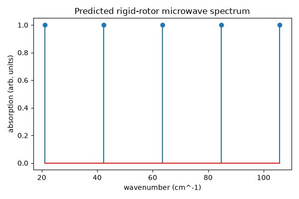
Transition spacings (should all equal 2B): [21.16834842 21.16834842 21.16834842 21.16834842]