Schrodinger’s hydrogen atom: radial wavefunctions and orbital energies

Schrodinger’s first 1926 paper solved his wave equation for the hydrogen atom and recovered the Bohr energies \(E_n\propto-1/n^2\) without any quantization postulate. HydrogenLikeAtom reproduces the textbook 13.6 eV hydrogen ground-state energy exactly, and its radial wavefunctions (built from the associated Laguerre polynomials of scipy.special) are independently checked here by numerically integrating them to a normalized probability of 1.

import matplotlib.pyplot as plt
import numpy as np

from chemistrykit.constants import ELECTRONVOLT
from chemistrykit.quantum.systems.hydrogenlike import HydrogenLikeAtom
from chemistrykit.quantum.visualizers.quantum_plots import plot_radial_distribution

h_atom = HydrogenLikeAtom(Z=1)
print(f"Bohr radius a0 = {h_atom.bohr_radius:.6e} m")
for n in (1, 2, 3, 4):
    print(f"E_{n} = {-h_atom.energy(n) / ELECTRONVOLT:.4f} eV (ionization energy from level n)")

Bohr radius a0 = 5.291772e-11 m
E_1 = 13.6057 eV (ionization energy from level n)
E_2 = 3.4014 eV (ionization energy from level n)
E_3 = 1.5117 eV (ionization energy from level n)
E_4 = 0.8504 eV (ionization energy from level n)

Every radial wavefunction should integrate (as r^2 R^2) to exactly 1 – a formula-agnostic sanity check independent of any particular associated-Laguerre-polynomial normalization convention:

for n, l in [(1, 0), (2, 0), (2, 1), (3, 0), (3, 1), (3, 2)]:
    norm = h_atom.check_radial_normalization(n, l)
    print(f"n={n}, l={l}: integral of r^2 R_nl(r)^2 dr = {norm:.6f}")

n=1, l=0: integral of r^2 R_nl(r)^2 dr = 1.000000
n=2, l=0: integral of r^2 R_nl(r)^2 dr = 1.000000
n=2, l=1: integral of r^2 R_nl(r)^2 dr = 1.000000
n=3, l=0: integral of r^2 R_nl(r)^2 dr = 1.000000
n=3, l=1: integral of r^2 R_nl(r)^2 dr = 1.000000
n=3, l=2: integral of r^2 R_nl(r)^2 dr = 1.000000

fig, ax = plt.subplots(figsize=(7, 5))
for n, l, style in [(1, 0, "-"), (2, 0, "--"), (2, 1, "-."), (3, 2, ":")]:
    plot_radial_distribution(h_atom, n, l, ax=ax, r_max_bohr_radii=25.0, linestyle=style, label=f"n={n}, l={l}")
ax.legend()
ax.set_title("Hydrogen radial distribution functions")
fig.tight_layout()

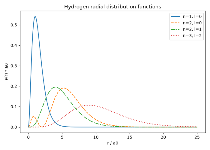
The 1s radial distribution function peaks at exactly r = a0 – the famous result that the Bohr-model “orbit radius” is really the most probable radial distance in the full quantum treatment, not a literal orbit:

a0 = h_atom.bohr_radius
r = np.linspace(1.0e-4 * a0, 6.0 * a0, 2000)
P = h_atom.radial_distribution_function(r, n=1, l=0)
r_peak = r[np.argmax(P)]
print(f"1s radial distribution peaks at r = {r_peak / a0:.4f} * a0 (expected: 1.0)")

plt.show()

1s radial distribution peaks at r = 0.9996 * a0 (expected: 1.0)