Harmonic vs. Morse vibrational levels: anharmonicity toward dissociation

Compares QuantumHarmonicOscillator’s perfectly evenly spaced levels against MorseOscillator’s exact (anharmonic) levels at the same force constant (compare_harmonic_vs_morse()), using HCl-like parameters, and shows the harmonic-oscillator ground-state wavefunction.

import matplotlib.pyplot as plt
import numpy as np
import scipy.constants as sc

from chemistrykit.quantum.systems.harmonic_oscillator import MorseOscillator, QuantumHarmonicOscillator, compare_harmonic_vs_morse
from chemistrykit.quantum.visualizers.quantum_plots import plot_harmonic_vs_morse_levels

# HCl-like reduced mass, force constant (~516 N/m matches the observed
# 2990 cm^-1 fundamental), and dissociation energy (~4.43 eV from the
# bottom of the well).
mu = (1.008 * sc.atomic_mass * 34.97 * sc.atomic_mass) / (1.008 * sc.atomic_mass + 34.97 * sc.atomic_mass)
k = 516.0
De = 4.43 * sc.eV

harmonic = QuantumHarmonicOscillator(mass=mu, force_constant=k)
morse = MorseOscillator(mass=mu, force_constant=k, dissociation_energy=De)
print(f"omega = {harmonic.angular_frequency:.4e} rad/s")
print(f"Morse anharmonicity constant x_e = {morse.anharmonicity_constant:.5f}")
print(f"Highest bound vibrational level v_max = {morse.v_max}")

omega = 5.6317e+14 rad/s
Morse anharmonicity constant x_e = 0.02092
Highest bound vibrational level v_max = 23

v_max_to_plot = 20
v, E_harmonic, E_morse = compare_harmonic_vs_morse(mass=mu, force_constant=k, dissociation_energy=De, v_max=v_max_to_plot)

fig, ax = plt.subplots(figsize=(7, 5))
plot_harmonic_vs_morse_levels(v, E_harmonic / sc.eV, E_morse / sc.eV, ax=ax)
ax.set_ylabel("energy (eV)")
ax.set_title("HCl-like oscillator: harmonic vs. Morse vibrational levels")
fig.tight_layout()

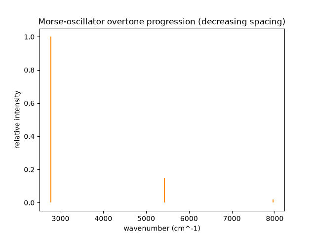
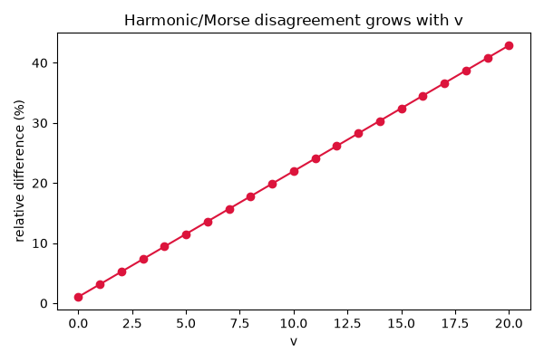
The two models agree closely at low v (where the Morse potential is well approximated by its harmonic term) but diverge as v grows – the Morse spacing shrinks toward dissociation while the harmonic spacing never changes:

relative_diff = np.abs(E_harmonic - E_morse) / E_harmonic
fig2, ax2 = plt.subplots(figsize=(6, 4))
ax2.plot(v, relative_diff * 100.0, "o-", color="crimson")
ax2.set_xlabel("v")
ax2.set_ylabel("relative difference (%)")
ax2.set_title("Harmonic/Morse disagreement grows with v")
fig2.tight_layout()

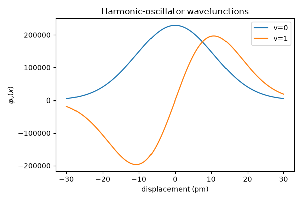
The harmonic-oscillator ground-state wavefunction is a simple Gaussian centered on the equilibrium bond length:

x = np.linspace(-3.0e-11, 3.0e-11, 400)
fig3, ax3 = plt.subplots(figsize=(6, 4))
ax3.plot(x * 1.0e12, harmonic.wavefunction(x, v=0), label="v=0")
ax3.plot(x * 1.0e12, harmonic.wavefunction(x, v=1), label="v=1")
ax3.set_xlabel("displacement (pm)")
ax3.set_ylabel(r"$\psi_v(x)$")
ax3.set_title("Harmonic-oscillator wavefunctions")
ax3.legend()
fig3.tight_layout()

plt.show()