Kuhn’s free-electron model of conjugated dye color

Hans Kuhn (1949) treated the pi electrons of a linear conjugated dye as free electrons in a one-dimensional box as long as the conjugated chain. With \(N\) pi electrons filling the box levels two at a time, the lowest absorption is the HOMO to LUMO jump, \(\Delta E=\frac{h^2}{8mL^2}(N+1)\), so a longer chain (more electrons and a longer box) absorbs at longer wavelength. conjugated_dye_absorption_wavelength() implements this on top of ParticleInBox1D.

import matplotlib.pyplot as plt
import numpy as np

from chemistrykit.constants import ELECTRONVOLT
from chemistrykit.quantum.systems.particle_in_box import ParticleInBox1D, conjugated_dye_absorption_wavelength

# A cyanine-like chain: 10 pi electrons in a 1.2 nm box.
L, n_pi = 1.2e-9, 10
box = ParticleInBox1D(length=L)
homo, lumo = n_pi // 2, n_pi // 2 + 1
wavelength = conjugated_dye_absorption_wavelength(box_length=L, n_pi_electrons=n_pi)
print(f"HOMO n={homo}, LUMO n={lumo}, gap = {(box.energy(lumo) - box.energy(homo)) / ELECTRONVOLT:.3f} eV")
print(f"predicted absorption: {wavelength * 1e9:.0f} nm")

fig, ax = plt.subplots(figsize=(5, 5))
for n in range(1, 9):
    E = box.energy(n) / ELECTRONVOLT
    ax.hlines(E, 0.0, 1.0, color="black" if n <= homo else "gray")
    if n <= homo:
        ax.text(0.5, E, "↑↓", ha="center", va="bottom", fontsize=11, color="steelblue")
ax.annotate(
    "",
    xy=(0.8, box.energy(lumo) / ELECTRONVOLT),
    xytext=(0.8, box.energy(homo) / ELECTRONVOLT),
    arrowprops={"arrowstyle": "->", "color": "crimson"},
)
ax.text(0.83, 0.5 * (box.energy(lumo) + box.energy(homo)) / ELECTRONVOLT, f"{wavelength * 1e9:.0f} nm", color="crimson")
ax.set_xticks([])
ax.set_ylabel("energy (eV)")
ax.set_title("Kuhn model: 10 pi electrons in a 1.2 nm box")
fig.tight_layout()

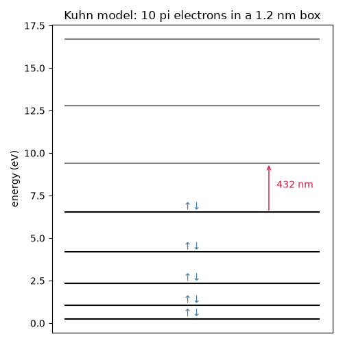
HOMO n=5, LUMO n=6, gap = 2.872 eV
predicted absorption: 432 nm

Lengthening the conjugated chain: each added C=C unit adds two pi electrons and roughly 0.28 nm of box, red-shifting the absorption.

electron_counts = np.arange(6, 22, 2)
lengths = 0.56e-9 + 0.14e-9 * (electron_counts - 6)
wavelengths_nm = [conjugated_dye_absorption_wavelength(box_length=Lk, n_pi_electrons=int(n)) * 1e9 for Lk, n in zip(lengths, electron_counts)]
for n, Lk, wl in zip(electron_counts, lengths, wavelengths_nm):
    print(f"{n:2d} pi electrons, L = {Lk * 1e9:.2f} nm -> lambda = {wl:.0f} nm")

fig2, ax2 = plt.subplots(figsize=(6, 4))
ax2.plot(electron_counts, wavelengths_nm, "o-", color="darkorange")
ax2.axhspan(400, 700, color="gold", alpha=0.15, label="visible range")
ax2.set_xlabel("number of pi electrons")
ax2.set_ylabel("predicted absorption wavelength (nm)")
ax2.set_title("Kuhn free-electron model: longer conjugation red-shifts absorption")
ax2.legend()
fig2.tight_layout()

plt.show()

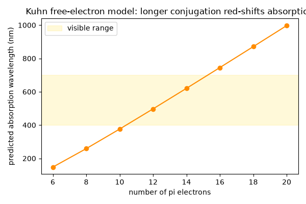
 6 pi electrons, L = 0.56 nm -> lambda = 148 nm
 8 pi electrons, L = 0.84 nm -> lambda = 258 nm
10 pi electrons, L = 1.12 nm -> lambda = 376 nm
12 pi electrons, L = 1.40 nm -> lambda = 497 nm
14 pi electrons, L = 1.68 nm -> lambda = 620 nm
16 pi electrons, L = 1.96 nm -> lambda = 745 nm
18 pi electrons, L = 2.24 nm -> lambda = 871 nm
20 pi electrons, L = 2.52 nm -> lambda = 997 nm