Kellner and Hylleraas: the variational helium atom and its screened charge

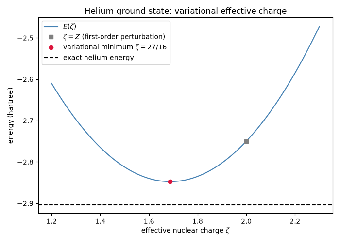
Helium was the first test of quantum mechanics beyond one electron. Kellner (1927) and Hylleraas (1928-1929) attacked it with the variational method: take both electrons in hydrogen-like 1s orbitals but let the nuclear charge they “see” be an adjustable \(\zeta\). The energy \(E(\zeta)=(\zeta^2-2Z\zeta+\tfrac{5}{8}\zeta)E_h\) (helium_like_variational_energy()) is lowest at \(\zeta=Z-5/16=27/16\) for helium (optimize_helium_like_effective_charge()): each electron shields the other from 5/16 of a nuclear charge. The result, \(-2.848\,E_h\), is within 2% of the exact \(-2.9037\,E_h\), which Hylleraas approached by adding the interelectronic distance to the trial function.

import matplotlib.pyplot as plt
import numpy as np

from chemistrykit.constants import ELECTRONVOLT
from chemistrykit.quantum.systems.helium import HARTREE_ENERGY, helium_like_variational_energy, optimize_helium_like_effective_charge

EXACT_HE = -2.903724  # nonrelativistic helium ground state, hartree
result = optimize_helium_like_effective_charge(2)
print(f"optimal zeta = {result.effective_charge} (screening constant {result.screening_constant})")
print(f"no e-e repulsion:        {result.independent_electron_energy / HARTREE_ENERGY:.4f} hartree")
print(f"first-order (zeta = Z):  {result.first_order_energy / HARTREE_ENERGY:.4f} hartree")
print(f"variational (zeta*):     {result.energy / HARTREE_ENERGY:.4f} hartree")
print(f"exact:                   {EXACT_HE:.4f} hartree")
print(f"first ionization energy: {result.ionization_energy / ELECTRONVOLT:.2f} eV (experiment 24.59 eV)")

zeta = np.linspace(1.2, 2.3, 300)
fig, ax = plt.subplots(figsize=(7, 5))
ax.plot(zeta, helium_like_variational_energy(zeta, Z=2) / HARTREE_ENERGY, color="steelblue", label=r"$E(\zeta)$")
ax.plot(2.0, result.first_order_energy / HARTREE_ENERGY, "s", color="gray", label=r"$\zeta=Z$ (first-order perturbation)")
ax.plot(result.effective_charge, result.energy / HARTREE_ENERGY, "o", color="crimson", label=r"variational minimum $\zeta=27/16$")
ax.axhline(EXACT_HE, color="black", linestyle="--", label="exact helium energy")
ax.set_xlabel(r"effective nuclear charge $\zeta$")
ax.set_ylabel("energy (hartree)")
ax.set_title("Helium ground state: variational effective charge")
ax.legend()
fig.tight_layout()

optimal zeta = 1.6875 (screening constant 0.3125)
no e-e repulsion:        -4.0000 hartree
first-order (zeta = Z):  -2.7500 hartree
variational (zeta*):     -2.8477 hartree
exact:                   -2.9037 hartree
first ionization energy: 23.07 eV (experiment 24.59 eV)

The same screening across the two-electron isoelectronic series. The relative error shrinks as Z grows (electron repulsion matters less), and for H- the simple trial function lies above the hydrogen atom plus a free electron (-0.5 hartree), wrongly predicting H- unbound; Bethe and Hylleraas (1929-1930) showed with correlated trial functions that it is in fact bound.

exact = {1: -0.527751, 2: -2.903724, 3: -7.279913, 4: -13.655566, 5: -22.030972}
names = {1: "H-", 2: "He", 3: "Li+", 4: "Be2+", 5: "B3+"}
Zs = np.array(sorted(exact))
variational = np.array([optimize_helium_like_effective_charge(Z).energy / HARTREE_ENERGY for Z in Zs])
errors = 100.0 * (variational - np.array([exact[Z] for Z in Zs])) / np.abs([exact[Z] for Z in Zs])
for Z, v, err in zip(Zs, variational, errors):
    print(f"{names[Z]:5s} Z={Z}: variational {v:9.4f}, exact {exact[Z]:9.4f} hartree ({err:.2f}% high)")

fig2, ax2 = plt.subplots(figsize=(6, 4))
ax2.bar([names[Z] for Z in Zs], errors, color="darkorange")
ax2.set_ylabel("variational energy error (%)")
ax2.set_title(r"Screened-charge helium-like ions: error vs. nuclear charge")
fig2.tight_layout()

plt.show()

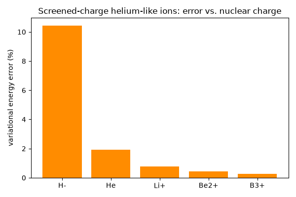
H-    Z=1: variational   -0.4727, exact   -0.5278 hartree (10.44% high)
He    Z=2: variational   -2.8477, exact   -2.9037 hartree (1.93% high)
Li+   Z=3: variational   -7.2227, exact   -7.2799 hartree (0.79% high)
Be2+  Z=4: variational  -13.5977, exact  -13.6556 hartree (0.42% high)
B3+   Z=5: variational  -21.9727, exact  -22.0310 hartree (0.26% high)