Coulson’s polyene formula and the Frost circle

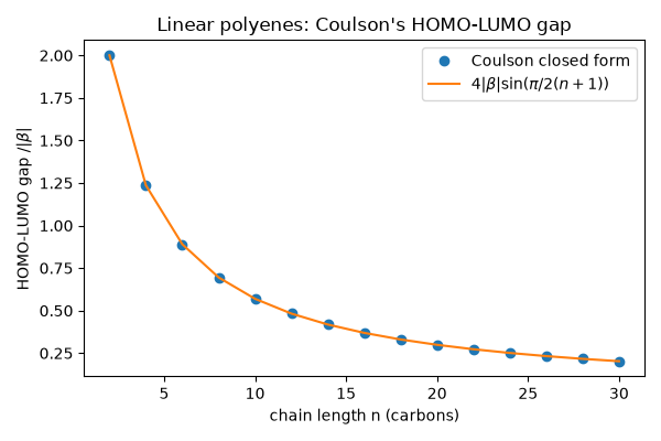
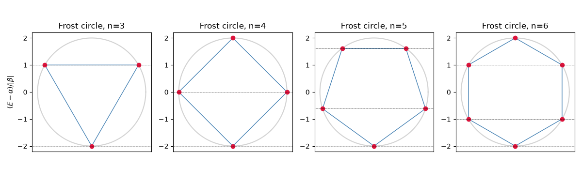
Coulson (1939) wrote the Huckel eigenvalues of a linear chain of n atoms in closed form, \(E_k=\alpha+2\beta\cos(k\pi/(n+1))\), and Frost and Musulin (1953) turned the ring result \(E_k=\alpha+2\beta\cos(2\pi k/n)\) into a drawing: put a regular n-gon, one vertex pointing down, inside a circle of radius \(2|\beta|\); the heights of the vertices are the orbital energies. Both closed forms (linear_polyene_eigenvalues(), cyclic_polyene_eigenvalues()) are checked here against numerical diagonalization.

import matplotlib.pyplot as plt
import numpy as np

from chemistrykit.quantum.systems.huckel import HuckelSystem, cyclic_polyene_eigenvalues, linear_polyene_eigenvalues

fig, axes = plt.subplots(1, 4, figsize=(12, 3.8))
theta = np.linspace(0.0, 2.0 * np.pi, 200)
for ax, n in zip(axes, (3, 4, 5, 6)):
    numeric = np.sort(HuckelSystem.cyclic_polyene(n).solve().energies)
    closed = cyclic_polyene_eigenvalues(n)
    print(f"ring n={n}: max |numeric - Frost| = {np.max(np.abs(numeric - closed)):.1e}")
    # vertex k at angle -pi/2 + 2 pi k / n, radius 2|beta|; height = energy (beta=-1)
    angles = -np.pi / 2.0 + 2.0 * np.pi * np.arange(n) / n
    x, y = 2.0 * np.cos(angles), 2.0 * np.sin(angles)
    ax.plot(2.0 * np.cos(theta), 2.0 * np.sin(theta), color="lightgray")
    ax.fill(x, y, facecolor="none", edgecolor="steelblue")
    ax.plot(x, y, "o", color="crimson")
    for e in numeric:
        ax.axhline(e, color="black", linewidth=0.4, linestyle=":")
    ax.set_aspect("equal")
    ax.set_title(f"Frost circle, n={n}")
    ax.set_xticks([])
axes[0].set_ylabel(r"$(E-\alpha)/|\beta|$")
fig.tight_layout()

ring n=3: max |numeric - Frost| = 4.4e-16
ring n=4: max |numeric - Frost| = 5.0e-16
ring n=5: max |numeric - Frost| = 4.4e-16
ring n=6: max |numeric - Frost| = 1.3e-15

Coulson’s linear-chain formula against diagonalization, and the HOMO-LUMO gap it predicts, \(4|\beta|\sin(\pi/(2(n+1)))\) for even n, shrinking toward zero for long chains.

n_values = np.arange(2, 31, 2)
gaps, errors = [], []
for n in n_values:
    numeric = np.sort(HuckelSystem.linear_polyene(n).solve().energies)
    closed = linear_polyene_eigenvalues(n)
    errors.append(np.max(np.abs(numeric - closed)))
    gaps.append(closed[n // 2] - closed[n // 2 - 1])
print(f"largest Coulson-formula deviation over n=2..30: {max(errors):.1e}")

fig2, ax2 = plt.subplots(figsize=(6, 4))
ax2.plot(n_values, gaps, "o", label="Coulson closed form")
ax2.plot(n_values, 4.0 * np.sin(np.pi / (2.0 * (n_values + 1))), "-", label=r"$4|\beta|\sin(\pi/2(n+1))$")
ax2.set_xlabel("chain length n (carbons)")
ax2.set_ylabel(r"HOMO-LUMO gap $/|\beta|$")
ax2.set_title("Linear polyenes: Coulson's HOMO-LUMO gap")
ax2.legend()
fig2.tight_layout()

plt.show()

largest Coulson-formula deviation over n=2..30: 1.8e-15