Fukui’s frontier orbitals: why naphthalene reacts at the alpha position

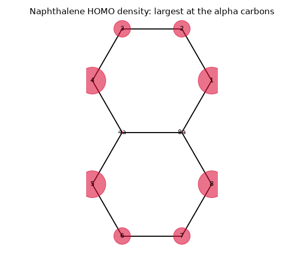
Kenichi Fukui, Teijiro Yonezawa and Haruo Shingu (1952) proposed that an aromatic hydrocarbon’s site of electrophilic substitution is set by one orbital alone, the highest occupied molecular orbital: the attacking electrophile goes where the HOMO density \(2c_r^2\) is largest. For naphthalene the Huckel HOMO has coefficient 0.425 on the alpha carbons (1, 4, 5, 8), 0.263 on the beta carbons (2, 3, 6, 7), and zero on the bridgeheads, so frontier_electron_density() predicts alpha substitution, which is what nitration and halogenation mostly give.

import matplotlib.pyplot as plt
import numpy as np

from chemistrykit.quantum.systems.huckel import HuckelSystem

# Atom order: C1, C2, C3, C4, C4a, C5, C6, C7, C8, C8a.
labels = ["1", "2", "3", "4", "4a", "5", "6", "7", "8", "8a"]
bonds = [(0, 1), (1, 2), (2, 3), (3, 4), (4, 5), (5, 6), (6, 7), (7, 8), (8, 9), (9, 0), (4, 9)]
naphthalene = HuckelSystem(n_atoms=10, bonds=bonds, labels=labels)

homo_density = naphthalene.frontier_electron_density(10, "homo")
for label, f in zip(labels, homo_density):
    print(f"C{label:3s} HOMO density = {f:.3f}")

C1   HOMO density = 0.362
C2   HOMO density = 0.138
C3   HOMO density = 0.138
C4   HOMO density = 0.362
C4a  HOMO density = 0.000
C5   HOMO density = 0.362
C6   HOMO density = 0.138
C7   HOMO density = 0.138
C8   HOMO density = 0.362
C8a  HOMO density = 0.000

Draw the molecule with circles proportional to the HOMO density.

s3 = np.sqrt(3.0) / 2.0
xy = np.array(
    [
        [-s3, 1.5],  # 1
        [-2 * s3, 1.0],  # 2
        [-2 * s3, 0.0],  # 3
        [-s3, -0.5],  # 4
        [0.0, 0.0],  # 4a
        [s3, -0.5],  # 5
        [2 * s3, 0.0],  # 6
        [2 * s3, 1.0],  # 7
        [s3, 1.5],  # 8
        [0.0, 1.0],  # 8a
    ]
)
xy = xy[:, ::-1] * np.array([1.0, -1.0])  # lay the molecule on its side

fig, ax = plt.subplots(figsize=(6, 5))
for i, j in bonds:
    ax.plot(xy[[i, j], 0], xy[[i, j], 1], color="black", linewidth=1.5)
ax.scatter(xy[:, 0], xy[:, 1], s=4000 * homo_density + 5, color="crimson", alpha=0.6, zorder=3)
for (x, y), label in zip(xy, labels):
    ax.text(x, y, label, ha="center", va="center", fontsize=9, zorder=4)
ax.set_aspect("equal")
ax.axis("off")
ax.set_title("Naphthalene HOMO density: largest at the alpha carbons")
fig.tight_layout()

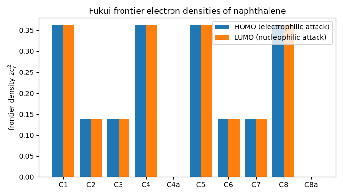
The LUMO has the same magnitudes (naphthalene is an alternant hydrocarbon), so nucleophilic and radical attack are predicted at the alpha positions too.

lumo_density = naphthalene.frontier_electron_density(10, "lumo")
fig2, ax2 = plt.subplots(figsize=(7, 4))
x = np.arange(10)
ax2.bar(x - 0.2, homo_density, width=0.4, label="HOMO (electrophilic attack)")
ax2.bar(x + 0.2, lumo_density, width=0.4, label="LUMO (nucleophilic attack)")
ax2.set_xticks(x)
ax2.set_xticklabels([f"C{lab}" for lab in labels])
ax2.set_ylabel(r"frontier density $2c_r^2$")
ax2.set_title("Fukui frontier electron densities of naphthalene")
ax2.legend()
fig2.tight_layout()

plt.show()