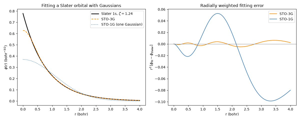
Hehre, Stewart and Pople’s STO-3G basis: three Gaussians for one Slater orbital

A Slater 1s orbital \(e^{-\zeta r}\) has the right cusp and tail but awkward integrals; a Gaussian has easy integrals but the wrong shape. STO-3G (sto3g_1s()) fixes three Gaussian exponents and coefficients by a least-squares fit to the Slater function once, for \(\zeta=1\). Every other exponent follows by scaling the Gaussian exponents by \(\zeta^2\). Below, the STO-3G contraction for hydrogen in molecules (\(\zeta=1.24\)) is compared with its Slater target and with a single best-fit Gaussian. The error concentrates at the nucleus and in the tail, but the region that matters for bonding is reproduced well.

import matplotlib.pyplot as plt
import numpy as np

from chemistrykit.quantum import RestrictedHartreeFock
from chemistrykit.quantum.systems.helium import HARTREE_ENERGY
from chemistrykit.quantum.utils.basis_sets import BOHR_RADIUS, sto3g_1s

zeta = 1.24
r = np.linspace(0.0, 4.0, 400)  # bohr
slater = (zeta**3 / np.pi) ** 0.5 * np.exp(-zeta * r)

phi = sto3g_1s(zeta, [0.0, 0.0, 0.0])
alphas = np.array([p.alpha for p in phi.primitives]) * BOHR_RADIUS**2  # back to bohr^-2
norms = (2 * alphas / np.pi) ** 0.75
sto3g = sum(d * n * np.exp(-a * r**2) for d, n, a in zip(phi.coefficients, norms, alphas, strict=True))

alpha_1g = 0.270950 * zeta**2  # STO-1G exponent (Szabo & Ostlund, eq. 3.221)
sto1g = (2 * alpha_1g / np.pi) ** 0.75 * np.exp(-alpha_1g * r**2)

fig, axes = plt.subplots(1, 2, figsize=(12, 4.8))
axes[0].plot(r, slater, color="black", linewidth=2, label=r"Slater 1s, $\zeta=1.24$")
axes[0].plot(r, sto3g, "--", color="darkorange", label="STO-3G")
axes[0].plot(r, sto1g, ":", color="steelblue", label="STO-1G (one Gaussian)")
axes[0].set_xlabel("r (bohr)")
axes[0].set_ylabel(r"$\phi(r)$ (bohr$^{-3/2}$)")
axes[0].set_title("Fitting a Slater orbital with Gaussians")
axes[0].legend()

axes[1].plot(r, r**2 * (sto3g - slater), color="darkorange", label="STO-3G")
axes[1].plot(r, r**2 * (sto1g - slater), color="steelblue", label="STO-1G")
axes[1].axhline(0.0, color="gray", linewidth=0.8)
axes[1].set_xlabel("r (bohr)")
axes[1].set_ylabel(r"$r^2\,[\phi_{fit}-\phi_{Slater}]$")
axes[1].set_title("Radially weighted fitting error")
axes[1].legend()
fig.tight_layout()

The same fitted contraction, rescaled for helium (\(\zeta=2.0925\)), reproduces Szabo & Ostlund’s minimal-basis results:

for name, rhf, reference in (("H2", RestrictedHartreeFock.h2(), -1.1167), ("HeH+", RestrictedHartreeFock.heh_plus(), -2.8607)):
    print(f"{name:5s} STO-3G RHF energy: {rhf.scf().total_energy / HARTREE_ENERGY:.4f} hartree (Szabo & Ostlund: {reference})")

plt.show()

H2    STO-3G RHF energy: -1.1167 hartree (Szabo & Ostlund: -1.1167)
HeH+  STO-3G RHF energy: -2.8607 hartree (Szabo & Ostlund: -2.8607)