
Breakthroughs in Photochemistry#
“Rays which are not absorbed produce no chemical action.” – attributed to J. W. Draper’s 1842-1843 statement of what is now called the Grotthuss-Draper law
Photochemistry asks what happens after a molecule absorbs a photon: not
whether a reaction is thermodynamically favorable, but which one of
several competing physical and chemical fates – fluorescence,
phosphorescence, heat, or genuine chemical change – claims the resulting
excited state, and how fast. The systems in chemistrykit.photochem
retrace the century and a half it took to turn that question into a
quantitative science: from the first statement that only absorbed light
does anything at all, through the photon-counting law of photochemical
equivalence and its most striking exception, to the Jablonski diagram
that organizes every excited-state fate into one picture, and the
photostationary state a molecule reaches when two of those fates run in
opposite directions at once – along with the measurements that made the
field quantitative (the Stokes shift, fluorescence anisotropy, flash
photolysis, chemical actinometry) and the ways an excited molecule hands
its energy or an electron to a neighbor (Förster and Dexter energy
transfer, Rehm-Weller electron transfer). This chronology traces the major
breakthroughs behind the package, with a pointer to the corresponding
implementation at each stop.
1817, 1842 – Grotthuss and Draper: Only Absorbed Light Acts#
Christian Johann Dietrich (Theodor) von Grotthuss, better known for the proton-hopping “Grotthuss mechanism” of ionic conduction in water, proposed in 1817 what is now considered the first law of photochemistry: that a photochemical effect can only be produced by light the reacting substance actually absorbs, with any transmitted or reflected light doing nothing at all, however intense. The idea seems self-evident in retrospect but was a genuine, nontrivial claim at the time, and it went essentially unnoticed outside a small circle for a generation. John William Draper, working independently in the United States and apparently unaware of Grotthuss’s earlier statement, arrived at the identical principle in the early 1840s from his own studies of light’s chemical (as opposed to heating or illuminating) action, stating flatly that rays which are not absorbed produce no chemical action whatsoever. The combined result – now universally known as the Grotthuss-Draper law – is the starting axiom of all quantitative photochemistry: before asking how efficiently absorbed light drives a reaction, one first has to know how much light was absorbed in the first place, a quantity every later entry in this chronology depends on.
Implementation: photons_absorbed()
computes exactly this quantity – the absorbed photon flux
\(I_{abs}=I_0(1-10^{-A})\), via
transmittance() – and is
the quantity every quantum-yield calculation in this module divides by,
never the incident flux itself, precisely because the Grotthuss-Draper
law says only the absorbed portion can do anything.
References: T. Grotthuss, “Physisch-chemische Forschungen” (1817), as commonly credited with the first statement of the law in secondary photochemistry literature; a precise, independently verified primary citation for the 1817 statement has not been located. J. W. Draper, “On Some Analogies Between the Phenomena of the Chemical Rays and Those of Radiant Heat,” Philos. Mag. Ser. 3, 19, 195-210 (1841), and subsequent papers through 1843, commonly cited as the independent restatement that gives the law its modern name.
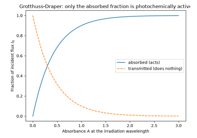
Grotthuss-Draper law: only absorbed light drives photochemistry
1852 – Stokes: Fluorescence Is Shifted to Longer Wavelength#
George Gabriel Stokes, investigating why a colorless solution of quinine glows blue when held in sunlight, dispersed the sunlight with a prism and found that only invisible ultraviolet rays beyond the violet end of the spectrum excited the glow – and that the blue light the solution emitted always had a longer wavelength than the light that produced it. He called the phenomenon “fluorescence” (after the mineral fluorspar) and stated the rule that bears his name: the emitted light is always of lower refrangibility, i.e. lower photon energy, than the absorbed light. The modern explanation is that an excited molecule loses part of its energy to vibrational relaxation and to reorganization of the surrounding solvent before it emits, so emission starts from a lower energy than absorption reached. The size of the gap – the Stokes shift – is still one of the first numbers reported for any new fluorophore, because a large shift lets the emitted light be separated cleanly from scattered excitation light.
Implementation: stokes_shift() returns
the shift in wavenumbers (cm-1) from the absorption and
emission maxima in nm, the energy-proportional unit in which Stokes
shifts are compared.
References: G. G. Stokes, “On the Change of Refrangibility of Light,” Phil. Trans. R. Soc. Lond. 142, 463-562 (1852).
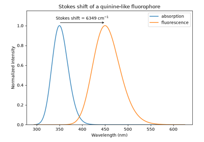
Stokes shift: fluorescence is emitted at longer wavelength than it is absorbed
1908, 1912 – 1913 – Stark, Einstein, and the Photochemical Equivalence Law#
Johannes Stark, in 1908, and Albert Einstein, working independently and from a different (thermodynamic) starting point in 1912-1913, each arrived at a sharper, quantitative version of the Grotthuss-Draper principle: not merely that only absorbed light acts, but that each individual quantum of absorbed light activates, at most, exactly one molecule. A priority dispute followed almost immediately – Einstein’s 1912 paper responds directly to a competing claim of priority from Stark – and the law is accordingly known today by both names, the Stark-Einstein law of photochemical equivalence. The principle gave photochemistry its first genuinely quantitative yardstick: dividing the amount of chemical product formed by the number of photons absorbed defines the quantum yield of a photoreaction, a number that should equal exactly 1 for the simplest possible case (one photon, one converted molecule, no competing pathway) – a natural reference point against which every real photoreaction’s efficiency, from a completely dark (non-absorbing, hence non-reacting) side reaction to the wildly super-unity yields of a radical chain reaction (see 1913-1918, below), could now be measured and compared.
Implementation: photochemical_quantum_yield()
implements exactly this ratio, \(\Phi=\) moles product formed /
moles photons absorbed; its doctest reproduces the simplest case the
Stark-Einstein law describes – one photon absorbed, one product molecule
formed, \(\Phi=1\) exactly – while its docstring explicitly flags
that a chain reaction can exceed this bound, the historically real
exception explored next.
References: J. Stark, Phys. Z. 9, 889-894 (1908) (page range as commonly cited in secondary literature; not independently verified); A. Einstein, “Thermodynamische Begründung des photochemischen Äquivalentgesetzes,” Ann. Phys. 37, 832-838 (1912); A. Einstein, “Antwort auf eine Bemerkung von J. Stark,” Ann. Phys. 38, 888 (1912), responding directly to Stark’s priority claim; A. Einstein, “Déduction thermodynamique de la loi de l’équivalence photochimique,” J. Phys. Théor. Appl. 3, 277-282 (1913).
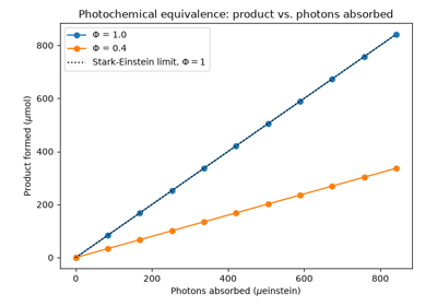
Stark-Einstein law: one absorbed photon, at most one reacting molecule
1913, 1918 – Bodenstein, Nernst, and the Photochemical Chain Reaction#
Max Bodenstein, measuring the quantum yield of the photochemical reaction between hydrogen and chlorine gas, found a result that flatly contradicted the brand-new Stark-Einstein law: rather than the expected yield of roughly 1, each absorbed photon was somehow responsible for the formation of on the order of \(10^5\)-\(10^6\) molecules of hydrogen chloride. Walther Nernst – better known for his electrochemical equation, and here contributing to photochemistry instead – proposed the resolution in 1918: a single absorbed photon splits one Cl2 molecule into two highly reactive chlorine atoms, and each atom then propagates a long chain of alternating reactions with H2 and Cl2, regenerating a fresh reactive chlorine atom at the end of every cycle and consuming thousands of H2/Cl2 pairs before the chain is finally broken by some termination step. The photochemical equivalence law was not wrong – each absorbed photon still activates only one molecule directly – but that single activation can, in a chain reaction, unleash an arbitrarily long cascade of further, purely thermal chemistry, giving an overall quantum yield with no upper bound at all.
Implementation: hydrogen_chlorine_chain_network()
builds Nernst’s mechanism – photolytic initiation
\(\mathrm{Cl_2}+h\nu\to2\,\mathrm{Cl}\), the two propagation steps
\(\mathrm{Cl}+\mathrm{H_2}\to\mathrm{HCl}+\mathrm{H}\) and
\(\mathrm{H}+\mathrm{Cl_2}\to\mathrm{HCl}+\mathrm{Cl}\), and
atom-recombination termination – as a
StoichiometricNetwork,
and chain_quantum_yield() gives the
steady-state quantum yield above, which grows without bound as the light
gets weaker (\(\Phi\propto I_{abs}^{-1/2}\)); this module’s tests
check that the integrated mechanism converges to it.
References: M. Bodenstein, “Eine Theorie der photochemischen Reaktionsgeschwindigkeiten,” Z. Phys. Chem. 85, 329-397 (1913); W. Nernst, “Zur Theorie der Reaktionsgeschwindigkeit in Gasen,” Z. Elektrochem. 24, 335-341 (1918) (chain-mechanism proposal for the H2/Cl2 system; page ranges for both papers are as commonly cited in secondary photochemistry literature and have not been independently verified against the original volumes).
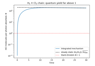
Bodenstein and Nernst: the H2 + Cl2 photochemical chain reaction
1919 – Stern and Volmer’s Quenching Equation#
Otto Stern and Max Volmer – the same Volmer who, a decade later, would help complete the Butler-Volmer equation in electrochemistry – studied how the presence of a second, “quencher” species suppresses a fluorescent molecule’s emission, by opening an additional nonradiative decay pathway (collisional energy transfer, electron transfer, or simply competing for the excitation) that competes with fluorescence for the excited-state population. They found the resulting suppression to be strikingly simple: the ratio of unquenched to quenched fluorescence intensity grows linearly with quencher concentration, with a slope (the Stern-Volmer constant) equal to the product of the quenching reaction’s bimolecular rate constant and the fluorophore’s own unquenched excited- state lifetime – a longer-lived excited state simply has more time to encounter a quencher molecule before it decays on its own. The same linear relationship, applied instead to the ratio of unquenched to quenched excited-state lifetimes, gives experimentalists a direct way to distinguish this genuinely dynamic (collisional) quenching mechanism from static quenching (pre-formed, non-fluorescent ground-state complexes), which suppresses intensity by the identical linear law while leaving the lifetime of whichever fluorophores remain uncomplexed completely unchanged.
Implementation: stern_volmer_ratio()
implements exactly this equation, and
dynamic_quenching_constant()
the \(K_{sv}=k_q\tau_0\) relationship for the dynamic case.
fit_stern_volmer()
recovers \(K_{sv}\) from synthetic intensity-ratio data by a
through-the-origin linear regression on the shift \(I_0/I-1\)
(the physically required zero-quencher intercept fixed at exactly 1
rather than left as a free-fit parameter), and
classify_quenching_mechanism()
implements the dynamic-vs-static diagnostic described above, comparing
the independently measured intensity-ratio and lifetime-ratio slopes.
References: O. Stern and M. Volmer, “Über die Abklingzeit der Fluoreszenz,” Phys. Z. 20, 183-188 (1919).
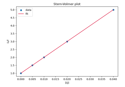
Stern-Volmer quenching, and distinguishing static from dynamic mechanisms
1920s – Vavilov’s Law of Constant Fluorescence Quantum Yield#
Sergei Vavilov, systematically measuring how a dye solution’s fluorescence quantum yield depends on the wavelength of the light used to excite it, found – after an initial 1922 study and further refinement through the mid-1920s – a result that is not at all obvious a priori: for a given fluorophore in a given environment, the fluorescence quantum yield is essentially independent of excitation wavelength, even though higher-energy (shorter-wavelength) photons deliver more excess energy to the molecule than lower-energy ones. The explanation, only fully systematized by Kasha’s rule three decades later (see 1950, below), is that whatever excited state absorption happens to populate directly, the molecule relaxes to the lowest excited state of that spin multiplicity before doing anything else (fluorescing, crossing to the triplet manifold, or decaying nonradiatively) – so the competition between those decay channels, and hence the resulting quantum yield, depends only on the rate constants out of that one lowest excited state, never on which higher state or vibrational level the exciting photon originally reached.
Implementation: fluorescence_quantum_yield()
is, by construction, a function purely of the three \(S_1\) decay
rate constants (\(\Phi_f=k_f/(k_f+k_{ic}+k_{isc})\)) and takes no
excitation-wavelength or excitation-energy parameter at all – exactly
Vavilov’s empirical law, encoded directly into the function’s signature
rather than merely satisfied numerically by some fortunate cancellation.
kasha_emission_yields() shows the same
result from the other side: exciting into a higher state \(S_2\)
changes the \(S_1\) fluorescence yield only by the factor
\(k_{ic,21}/(k_{f2}+k_{ic,21})\), indistinguishable from 1 for
typical rates.
References: S. I. Vavilov, “Die Fluoreszenzausbeute von Farbstofflösungen als Funktion der Wellenlänge des anregenden Lichtes,” Z. Phys. 42, 311-318 (1927), consolidating his earlier 1922 measurements (exact citation for the 1922 work not independently verified here).
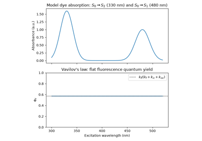
Vavilov’s law: fluorescence quantum yield is independent of excitation wavelength
1926 – Perrin’s Equation for Fluorescence Anisotropy#
Francis Perrin showed that the polarization of fluorescence carries a clock. A fluorophore excited by polarized light is excited preferentially when its absorption dipole lies along the light’s electric field, so its emission starts out polarized; but the molecule tumbles by rotational diffusion during its excited-state lifetime \(\tau\), and the longer it lives relative to its rotational correlation time \(\theta\), the more that polarization is lost. For a spherical molecule the steady-state anisotropy obeys a simple law, and since \(\theta=\eta V/k_BT\) depends on the solvent viscosity and the molecule’s volume, measuring the anisotropy reveals how large the emitting molecule (or the protein it is bound to) is, or how viscous its surroundings are. The same paper used depolarization to estimate excited-state lifetimes of nanoseconds, long before they could be timed directly.
Implementation: perrin_anisotropy()
evaluates the Perrin equation and
rotational_correlation_time() the
Stokes-Einstein-Debye correlation time; the tests check that a “Perrin
plot” of \(1/r\) against \(T/\eta\) is a straight line with
intercept \(1/r_0\).
References: F. Perrin, “Polarisation de la lumière de fluorescence. Vie moyenne des molécules dans l’état excité,” J. Phys. Radium 7, 390-401 (1926).
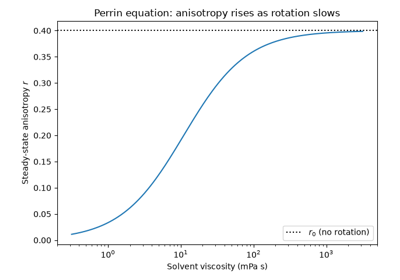
Perrin equation: fluorescence anisotropy and molecular rotation
1933 – Jablonski’s Diagram#
Aleksander Jablonski, a Polish physicist working on the polarization of fluorescence, introduced the energy-level diagram that now bears his name: a single organized picture of every radiative and nonradiative pathway available to a molecule after it absorbs a photon and lands in an excited electronic state – prompt fluorescence back to the ground state, radiationless internal conversion, intersystem crossing into the lower-energy but spin-forbidden (and hence much longer-lived) triplet manifold, and, from there, either slow phosphorescence or further nonradiative decay. What had been, before Jablonski, a scattered collection of separately named phenomena became, with his diagram, a single coherent kinetic scheme: every excited-state fate is just one more first-order (or, for intersystem crossing, still effectively unimolecular) rate process competing with all the others for the same finite excited- state population, exactly the same mass-action mathematics as an ordinary chemical reaction network.
Implementation: jablonski_network()
builds precisely this three-state (\(S_1\), \(T_1\), \(S_0\))
diagram directly as a
chemistrykit.kinetics.systems.networks.StoichiometricNetwork –
reusing the kinetics domain’s general mass-action reaction-network engine
rather than reimplementing rate-equation integration, since a Jablonski
diagram is, mathematically, nothing more than a branching-then-
consecutive first-order reaction network. jablonski_populations_analytic()
gives the closed-form Bateman-equation solution for all three
populations, checked in this module’s own test suite to agree with the
network’s numerical integration to better than \(10^{-10}\).
References: A. Jablonski, “Efficiency of Anti-Stokes Fluorescence in Dyes,” Nature 131, 839-840 (1933).
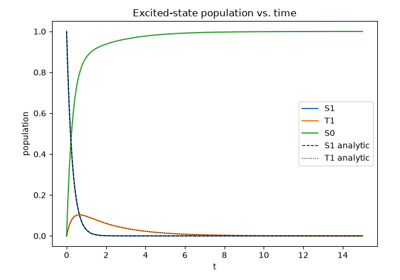
1944 – Lewis and Kasha: Phosphorescence as Triplet-State Emission#
For decades after phosphorescence was first distinguished experimentally from ordinary (prompt) fluorescence by its far longer afterglow, its physical origin remained genuinely mysterious – an anomalously long-lived, spin-forbidden emission with no settled explanation. Gilbert N. Lewis and Michael Kasha resolved the question in 1944: from spectroscopic and kinetic studies of organic molecules frozen in rigid glasses, they identified the phosphorescent state as the lowest triplet state – a state with two unpaired electron spins, rather than the ordinary, spin-paired singlet – and predicted that it should therefore be paramagnetic, which Lewis, Calvin, and Kasha confirmed by magnetic susceptibility measurements in 1949. Phosphorescence’s characteristic slowness followed immediately: emission from a triplet state back to the singlet ground state is spin-forbidden by the same selection rule that makes intersystem crossing itself a comparatively slow process, so a molecule that reaches the triplet manifold can linger there, on timescales of milliseconds to seconds rather than the nanoseconds typical of allowed fluorescent transitions, before it finally, reluctantly, emits.
Implementation: the \(T_1\) state in
jablonski_network() is
exactly the triplet state Lewis and Kasha identified, decaying at the
comparatively slow combined rate \(k_p+k_{ic,T}\); phosphorescence_quantum_yield()
computes the probability that an excited molecule both reaches this
triplet state (via intersystem_crossing_yield())
and then decays radiatively from it – the product of exactly the two
successive branching probabilities Lewis and Kasha’s triplet-state
picture implies.
References: G. N. Lewis and M. Kasha, “Phosphorescence and the Triplet State,” J. Am. Chem. Soc. 66, 2100-2116 (1944); G. N. Lewis, M. Calvin, and M. Kasha, “Photomagnetism. Determination of the Paramagnetic Susceptibility of a Dye in Its Phosphorescent State,” J. Chem. Phys. 17, 804 (1949).
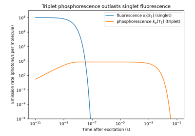
Lewis and Kasha: phosphorescence as slow emission from the triplet state
1948 – Förster Resonance Energy Transfer#
Theodor Förster gave the quantitative theory of how an excited molecule (the donor) can pass its excitation, without emitting a photon, to a different molecule (the acceptor) several nanometers away. The two molecules’ transition dipoles couple through their near fields, and Förster showed that the transfer rate falls off as the inverse sixth power of their separation and is proportional to the overlap between the donor’s emission spectrum and the acceptor’s absorption spectrum. All of the spectroscopy can be packed into one characteristic length, the Förster distance \(R_0\) (typically 2-8 nm) at which transfer and the donor’s own decay are equally fast. Because the efficiency changes from nearly 1 to nearly 0 over a narrow range around \(R_0\), Förster transfer (FRET) later became a “spectroscopic ruler” for distances inside proteins, nucleic acids, and membranes.
Implementation: forster_radius() computes
\(R_0\) from the orientation factor, refractive index, donor quantum
yield, and spectral overlap integral;
forster_rate() and
forster_efficiency() give the transfer rate
and efficiency.
References: Th. Förster, “Zwischenmolekulare Energiewanderung und Fluoreszenz,” Ann. Phys. 437 (6. Folge, 2), 55-75 (1948).
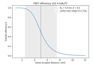
Förster resonance energy transfer: the inverse-sixth-power distance law
1949 – Norrish and Porter’s Flash Photolysis#
Every entry so far describes what happens to an excited molecule in principle; observing it directly, in real time, was a separate and much harder experimental problem, since the reactive intermediates a photoreaction produces – excited states, radicals, ions – typically survive for only microseconds or less. Ronald Norrish and George Porter solved it by turning the problem’s own difficulty into the tool: firing an intense flash lamp discharge to photolyze a sample far faster than its intermediates could decay, then probing the resulting transient absorption spectrum with a second, precisely delayed flash, they could watch a short-lived species appear and disappear on its own natural timescale for the first time, rather than inferring its existence indirectly from a reaction’s final products. Flash photolysis and its many later refinements (down to femtosecond pulses, decades afterward) turned photochemistry from a science of stable starting materials and stable products into one that can watch the unstable, fleeting intermediates in between – work recognized with a share, together with Manfred Eigen, of the 1967 Nobel Prize in Chemistry.
Implementation: flash photolysis is an experimental technique rather
than an algorithm, but its measurement is easy to simulate: the
time-resolved \(T_1(t)\) population from
jablonski_populations_analytic(), multiplied
by a triplet-triplet molar absorptivity and path length, is the transient
absorbance \(\Delta A(t)\) a delayed probe flash records, and a
log-linear fit of that decay recovers the triplet lifetime
\(1/(k_p+k_{ic,T})\).
References: R. G. W. Norrish and G. Porter, “Chemical Reactions Produced by Very High Light Intensities,” Nature 164, 658 (1949).
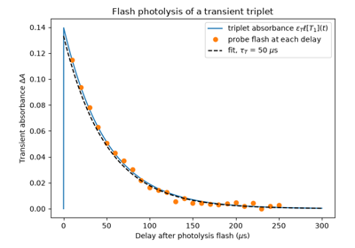
Norrish and Porter’s flash photolysis: watching a transient triplet decay
1950 – Kasha’s Rule#
Michael Kasha, four years after his triplet-state work with Lewis, proposed a second, more general organizing principle for excited-state photophysics: for a molecule excited to any electronic state, of any multiplicity, above the lowest excited state of that same multiplicity, internal conversion and vibrational relaxation to that lowest state happen so much faster than any radiative or further electronic-relaxation process that essentially all subsequent emission – fluorescence from the lowest excited singlet, phosphorescence from the lowest triplet – originates there and only there, regardless of which higher state absorption first populated. Kasha’s rule is what makes it physically sensible to model a molecule’s excited-state kinetics with just one representative singlet and one representative triplet level, as this package’s Jablonski-diagram model does, rather than needing to track every individual excited state a real absorption spectrum might reach: whichever \(S_n\) (\(n\ge2\)) a photon actually populates, Kasha’s rule guarantees it collapses to \(S_1\) before anything else of photochemical consequence happens.
Implementation: jablonski_network()’s
minimal three-state structure – exactly one representative singlet
excited state (\(S_1\)) and one representative triplet
(\(T_1\)), rather than a separate state for every electronic level a
real molecule’s absorption spectrum might access – is the direct
modeling consequence of Kasha’s rule: higher excited states are assumed
(correctly, for the overwhelming majority of molecules) to funnel down to
\(S_1\)/\(T_1\) before competing further, so the minimal model
loses no essential photophysics by omitting them.
kasha_emission_yields() makes the rule
quantitative for an \(S_2\)/\(S_1\) pair: the share of emission
from \(S_2\) is \(k_{f2}/(k_{f2}+k_{ic,21})\), of order
\(10^{-5}\) for typical internal-conversion rates, and becomes
appreciable only when \(S_2\to S_1\) conversion is unusually slow (the
famous exception, azulene).
References: M. Kasha, “Characterization of Electronic Transitions in Complex Molecules,” Discuss. Faraday Soc. 9, 14-19 (1950).
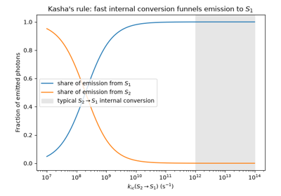
Kasha’s rule: emission comes from the lowest excited state
1953 – Dexter’s Exchange Mechanism of Energy Transfer#
David L. Dexter extended Förster’s theory to transitions that dipole coupling cannot drive efficiently – in particular to sensitized luminescence in solids involving forbidden transitions. In the exchange mechanism the donor and acceptor effectively swap electrons, which requires their electron clouds to overlap; the rate therefore decays exponentially with separation and is significant only within about 1 nm of contact, far shorter range than Förster transfer. Because electron exchange conserves total spin, it can carry triplet excitation from one molecule to another (triplet-triplet energy transfer), the basis of photosensitization, of triplet quenching by oxygen and dienes, and of the triplet sensitizers widely used in synthetic photochemistry.
Implementation: dexter_rate() evaluates
the exchange rate for a pre-exponential factor \(K\), normalized
spectral overlap \(J\), and effective van der Waals radius
\(L\).
References: D. L. Dexter, “A Theory of Sensitized Luminescence in Solids,” J. Chem. Phys. 21, 836-850 (1953).
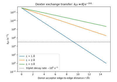
Dexter exchange energy transfer: exponential fall-off with distance
1956 – Hatchard and Parker’s Ferrioxalate Actinometer#
Every quantum yield in this chronology needs the number of photons absorbed, and measuring light intensity accurately in the ultraviolet and visible was, for decades, a major source of error. C. G. Hatchard and C. A. Parker introduced potassium ferrioxalate as a chemical actinometer – a reaction that counts photons. In acidic solution, light reduces Fe(III) in the ferrioxalate complex to Fe(II) with a quantum yield that they measured carefully across the UV and blue (about 1.2 in the near UV), and the Fe(II) formed is then determined very sensitively as its intensely red complex with 1,10-phenanthroline. The actinometer is sensitive, absorbs strongly over a wide wavelength range, and is easy to use, and it remains the standard way photochemists calibrate their light sources.
Implementation: ferrioxalate_fe2_moles()
converts the phenanthroline complex’s absorbance at 510 nm into moles of
Fe(II) (Beer-Lambert), and
ferrioxalate_photon_flux() turns that
into the photon flux using the equation above.
References: C. G. Hatchard and C. A. Parker, “A New Sensitive Chemical Actinometer. II. Potassium Ferrioxalate as a Standard Chemical Actinometer,” Proc. R. Soc. Lond. A 235, 518-536 (1956); H. J. Kuhn, S. E. Braslavsky, and R. Schmidt, “Chemical Actinometry (IUPAC Technical Report),” Pure Appl. Chem. 76, 2105-2146 (2004).
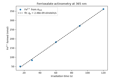
Hatchard and Parker’s ferrioxalate actinometer: counting photons chemically
1967 – Fischer and the Photostationary State#
A molecular photoswitch – two forms, A and B, each capable of absorbing the same irradiation wavelength and photoisomerizing to the other – behaves nothing like an ordinary photoreaction that simply runs to completion: under continuous illumination, both the forward and reverse photoreactions run simultaneously, and the system settles instead into a photostationary state (PSS), a genuinely dynamic (not thermodynamic) balance in which nonzero forward and reverse photon-driven isomerization rates happen to exactly cancel in the population balance. Egmont Fischer worked out the composition of this photostationary state in closed form directly from the two directions’ quantum yields and molar absorptivities, giving photochemists a simple algebraic target – the [B]/[A] ratio a given photoswitch and illumination wavelength will settle into – against which real photoswitching experiments (a widely used class of molecular tools, from azobenzenes to diarylethenes) could be quantitatively checked.
Implementation: photoswitch_rate_constants()
converts quantum yields and molar absorptivities into the pseudo-first-
order rate constants \(k_{AB}\), \(k_{BA}\) in Fischer’s
low-optical-density approximation;
photoswitch_network()
reuses reversible()
directly (a photoswitch under simultaneous forward/reverse photolysis
being, mathematically, the identical reversible first-order network a
thermally reversible reaction would be), and
photostationary_state()
gives Fischer’s exact algebraic PSS ratio
\([B]_{pss}/[A]_{pss}=k_{AB}/k_{BA}\) – checked in this module’s own
example against direct long-time numerical integration of the ODE
network, which converges to the identical ratio.
References: E. Fischer, “The Calculation of Photostationary States in Systems A <-> B When Only A is Known,” J. Phys. Chem. 71, 3704-3706 (1967).
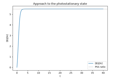
Photostationary-state kinetics of a two-state photoswitch
1970 – Rehm and Weller: Electron-Transfer Quenching#
Dieter Rehm and Albert Weller measured how quickly dozens of donor-acceptor pairs quench fluorescence by photoinduced electron transfer in acetonitrile and found that all their rate constants fell on a single curve when plotted against the free energy of the electron transfer. That free energy can be estimated from simple, independently measurable quantities: the donor’s oxidation potential, the acceptor’s reduction potential, the excitation energy \(E_{00}\) of whichever partner is excited, and a small Coulombic term. Quenching is diffusion-controlled when transfer is exergonic by more than a few tenths of an eV and falls off steeply when it is endergonic. The Rehm-Weller relation made it possible to predict whether an excited state will act as an oxidant or reductant toward a given partner, the basis of later photoredox catalysis. Their data did not show the “inverted region” predicted by Marcus theory at very high driving force, which was first observed clearly only in the 1980s.
Implementation: rehm_weller_free_energy()
computes \(\Delta G_{ET}\) and
rehm_weller_quenching_rate() the empirical
Rehm-Weller quenching rate constant, with the diffusion rate, rate-constant
ratio, and intrinsic barrier of the original acetonitrile fit as
defaults.
References: D. Rehm and A. Weller, “Kinetics of Fluorescence Quenching by Electron and H-Atom Transfer,” Isr. J. Chem. 8, 259-271 (1970).
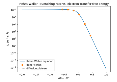
Rehm-Weller equation: electron-transfer quenching vs. driving force