Photostationary-state kinetics of a two-state photoswitch

A photoswitch A <-> B under simultaneous forward and reverse photolysis reaches a photostationary state (PSS) rather than running to completion. photoswitch_network() reuses reversible() directly, and photostationary_state() gives the exact algebraic PSS composition – checked here against direct long-time numerical integration of the ODE system.

import matplotlib.pyplot as plt

from chemistrykit.photochem.systems.photostationary_state import (
    photostationary_ratio,
    photostationary_state,
    photoswitch_network,
    photoswitch_rate_constants,
)
from chemistrykit.photochem.visualizers.photochem_plots import plot_photostationary_approach

Rate constants from quantum yields and molar absorptivities (the low-optical-density approximation – see the module docstring). The incident intensity I0 is left at a convenient normalized value (rather than a literal photon flux) so the resulting pseudo-first-order rate constants are O(1) on the plotted timescale below.

phi_AB, eps_A = 0.55, 1.8e4
phi_BA, eps_B = 0.30, 6.0e3
I0 = 1.0e-4
k_AB, k_BA = photoswitch_rate_constants(phi_AB, eps_A, phi_BA, eps_B, I0=I0)
print(f"k_AB = {k_AB:.4f}, k_BA = {k_BA:.4f}")

net = photoswitch_network(k_AB, k_BA, A0=1.0)
result = net.integrate((0.0, 40.0), dt=1e-2, method="rk4")

pss = photostationary_state(k_AB, k_BA, total_concentration=1.0)
print(f"\nPSS ratio [B]/[A] (algebraic):  {pss.ratio_B_over_A:.4f}")
print(f"PSS ratio [B]/[A] (long-time numeric): {result.concentration('B')[-1] / result.concentration('A')[-1]:.4f}")
print(f"Sanity check (Fischer's formula): {photostationary_ratio(k_AB, k_BA):.4f}")

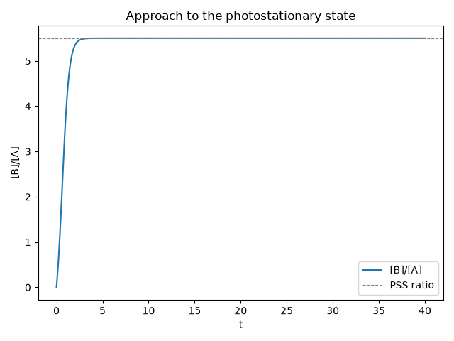
ax = plot_photostationary_approach(result, pss)
plt.tight_layout()
plt.show()

k_AB = 2.2800, k_BA = 0.4145

PSS ratio [B]/[A] (algebraic):  5.5000
PSS ratio [B]/[A] (long-time numeric): 5.5000
Sanity check (Fischer's formula): 5.5000