Perrin equation: fluorescence anisotropy and molecular rotation

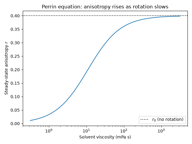
Perrin (1926) related the polarization of fluorescence to how far a molecule rotates during its excited-state lifetime \(\tau\): \(r=r_0/(1+\tau/\theta)\), with rotational correlation time \(\theta=\eta V/k_BT\) (perrin_anisotropy(), rotational_correlation_time()). A small dye depolarizes almost completely in water but stays polarized in viscous glycerol, and a “Perrin plot” of \(1/r\) against \(T/\eta\) is a straight line whose intercept gives \(r_0\) and whose slope gives the molecular volume.

import matplotlib.pyplot as plt
import numpy as np

from chemistrykit.constants import K_B
from chemistrykit.photochem import perrin_anisotropy, rotational_correlation_time

r0, tau = 0.4, 4.0e-9  # fundamental anisotropy, lifetime (s)
V = 1.5e-27  # hydrodynamic volume, m^3 (~1.5 nm^3)
T = 298.15
eta = np.logspace(-3.5, 0.5, 200)  # Pa*s, from below water to glycerol-like

r = perrin_anisotropy(r0, tau, rotational_correlation_time(eta, V, T))
fig, ax = plt.subplots()
ax.semilogx(eta * 1e3, r)
ax.axhline(r0, color="k", ls=":", label=r"$r_0$ (no rotation)")
ax.set_xlabel("Solvent viscosity (mPa s)")
ax.set_ylabel("Steady-state anisotropy $r$")
ax.set_title("Perrin equation: anisotropy rises as rotation slows")
ax.legend()
fig.tight_layout()

Perrin plot from synthetic measurements at several temperatures.

rng = np.random.default_rng(1)
T_meas = np.linspace(283.0, 333.0, 6)
eta_meas = 5.0e-3
r_meas = perrin_anisotropy(r0, tau, rotational_correlation_time(eta_meas, V, T_meas)) * (1 + rng.normal(0, 0.005, 6))
x = T_meas / eta_meas
# 1/r = 1/r0 + (tau k_B / (r0 V)) T/eta, so intercept = 1/r0 and V = intercept tau k_B / slope.
slope, intercept = np.polyfit(x, 1.0 / r_meas, 1)
V_fit = intercept * tau * K_B / slope
print(f"Fitted r0 = {1 / intercept:.3f} (true {r0}), fitted V = {V_fit * 1e27:.2f} nm^3 (true 1.50)")

fig2, ax2 = plt.subplots()
ax2.plot(x, 1.0 / r_meas, "o", label="measured")
ax2.plot(x, intercept + slope * x, "k--", label="linear fit")
ax2.set_xlabel(r"$T/\eta$ (K Pa$^{-1}$ s$^{-1}$)")
ax2.set_ylabel("$1/r$")
ax2.set_title("Perrin plot")
ax2.legend()
fig2.tight_layout()

plt.show()

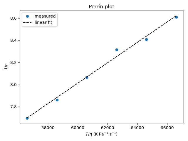
Fitted r0 = 0.405 (true 0.4), fitted V = 1.48 nm^3 (true 1.50)