Hatchard and Parker’s ferrioxalate actinometer: counting photons chemically

Every quantum yield needs the number of photons absorbed. Hatchard and Parker (1956) introduced potassium ferrioxalate as a sensitive chemical photon counter: light reduces Fe(III) to Fe(II) with a known quantum yield (about 1.21 at 365 nm), and the Fe(II) is measured by the red phenanthroline complex at 510 nm (ferrioxalate_fe2_moles()). Dividing by the quantum yield and the irradiation time gives the lamp’s photon flux (ferrioxalate_photon_flux()). 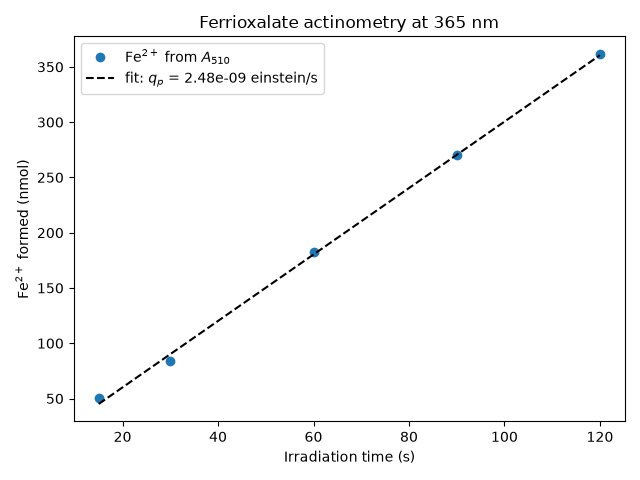Here synthetic readings from a series of irradiation times are converted back into the flux of a lamp of known output.

Flux from each exposure (einstein/s): [2.804e-09 2.310e-09 2.516e-09 2.486e-09 2.492e-09]
Flux from slope: 2.483e-09 einstein/s (true 2.500e-09)

import matplotlib.pyplot as plt
import numpy as np

from chemistrykit.photochem import ferrioxalate_fe2_moles, ferrioxalate_photon_flux

q_true = 2.5e-9  # einstein/s reaching the cell (unknown to the "experimenter")
Phi_Fe = 1.21
V_developed = 0.010  # L after adding phenanthroline and buffer
t = np.array([15.0, 30.0, 60.0, 90.0, 120.0])  # s

rng = np.random.default_rng(3)
n_fe2_true = Phi_Fe * q_true * t  # total absorption (concentrated actinometer)
A510 = n_fe2_true * 1.11e4 / V_developed + rng.normal(0.0, 0.003, t.size)

n_fe2 = ferrioxalate_fe2_moles(A510, V_developed)
q_each = ferrioxalate_photon_flux(n_fe2, t, quantum_yield=Phi_Fe)
slope = np.polyfit(t, n_fe2, 1)[0]
q_fit = ferrioxalate_photon_flux(slope, 1.0, quantum_yield=Phi_Fe)
print("Flux from each exposure (einstein/s):", np.array2string(q_each, precision=3))
print(f"Flux from slope: {q_fit:.3e} einstein/s (true {q_true:.3e})")

fig, ax = plt.subplots()
ax.plot(t, n_fe2 * 1e9, "o", label=r"Fe$^{2+}$ from $A_{510}$")
ax.plot(t, slope * t * 1e9, "k--", label=rf"fit: $q_p$ = {q_fit:.2e} einstein/s")
ax.set_xlabel("Irradiation time (s)")
ax.set_ylabel(r"Fe$^{2+}$ formed (nmol)")
ax.set_title("Ferrioxalate actinometry at 365 nm")
ax.legend()
fig.tight_layout()

plt.show()