Stark-Einstein law: one absorbed photon, at most one reacting molecule

The law of photochemical equivalence (Stark 1908, Einstein 1912-1913) says each absorbed quantum activates exactly one molecule. The quantum yield \(\Phi\) (moles product / moles photons absorbed), computed by photochemical_quantum_yield(), then equals 1 for an ideal one-photon, one-molecule reaction and is less than 1 when the excited molecule has other ways to lose its energy.

import matplotlib.pyplot as plt
import numpy as np

from chemistrykit.photochem import photochemical_quantum_yield, photons_absorbed

# Photons absorbed over a series of exposures (Beer-Lambert, A = 0.8).
I0, A = 1.0e-6, 0.8
t = np.linspace(0.0, 1000.0, 11)
n_photons = photons_absorbed(I0, A) * t

# Product formed if every activated molecule reacts (efficiency 1), or if
# 60% of activated molecules decay back without reacting.
fig, ax = plt.subplots()
for efficiency in (1.0, 0.4):
    n_product = efficiency * n_photons
    ax.plot(n_photons * 1e6, n_product * 1e6, "o-", label=rf"$\Phi$ = {efficiency}")
ax.plot(n_photons * 1e6, n_photons * 1e6, "k:", label=r"Stark-Einstein limit, $\Phi=1$")
ax.set_xlabel(r"Photons absorbed ($\mu$einstein)")
ax.set_ylabel(r"Product formed ($\mu$mol)")
ax.set_title("Photochemical equivalence: product vs. photons absorbed")
ax.legend()
fig.tight_layout()

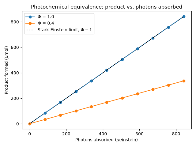
The quantum yield is the slope of that line.

Phi = photochemical_quantum_yield(0.4 * n_photons[1:], n_photons[1:])
print("Quantum yield at every exposure:", np.round(Phi, 6))

plt.show()

Quantum yield at every exposure: [0.4 0.4 0.4 0.4 0.4 0.4 0.4 0.4 0.4 0.4]