Jablonski-diagram excited-state kinetics

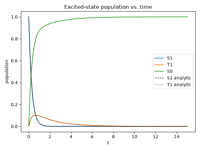
jablonski_network() builds the 3-state (S1, T1, S0) Jablonski excited-state decay network as a StoichiometricNetwork – reusing the kinetics domain’s general mass-action reaction-network engine rather than reimplementing rate-equation integration. The numerical integration is checked here against jablonski_populations_analytic()’s closed-form solution.

import matplotlib.pyplot as plt
import numpy as np

from chemistrykit.photochem.systems.jablonski import jablonski_network, jablonski_populations_analytic
from chemistrykit.photochem.visualizers.photochem_plots import plot_state_populations

kf, kic, kisc, kp, kic_T = 2.0, 1.0, 0.5, 0.3, 0.2
S1_0 = 1.0

net = jablonski_network(kf, kic, kisc, kp, kic_T, S1_0=S1_0)
result = net.integrate((0.0, 15.0), dt=1e-3, method="rk4")

S1_analytic, T1_analytic, S0_analytic = jablonski_populations_analytic(kf, kic, kisc, kp, kic_T, S1_0, result.t)
max_error = max(
    np.max(np.abs(result.concentration("S1") - S1_analytic)),
    np.max(np.abs(result.concentration("T1") - T1_analytic)),
    np.max(np.abs(result.concentration("S0") - S0_analytic)),
)
print(f"Max deviation between numerical and closed-form populations: {max_error:.2e}")

Max deviation between numerical and closed-form populations: 4.61e-13

ax = plot_state_populations(result)
ax.plot(result.t, S1_analytic, "k--", linewidth=1, label="S1 analytic")
ax.plot(result.t, T1_analytic, "k:", linewidth=1, label="T1 analytic")
ax.legend()
plt.tight_layout()

Quantum-yield-relevant quantities: the S1 total decay rate, and the fraction of excited molecules that ever populate the triplet state.

k_S1_total = kf + kic + kisc
isc_fraction = kisc / k_S1_total
print(f"\nTotal S1 decay rate: {k_S1_total:.3f}")
print(f"Fraction of excited S1 crossing to T1: {isc_fraction:.3f}")

plt.show()

Total S1 decay rate: 3.500
Fraction of excited S1 crossing to T1: 0.143