Rehm-Weller equation: electron-transfer quenching vs. driving force

Rehm and Weller (1970) measured how fast many donor-acceptor pairs quench fluorescence by electron transfer in acetonitrile and found that the quenching rate constant depends on a single quantity, the electron-transfer free energy \(\Delta G_{ET}=E_{ox}(D)-E_{red}(A)-E_{00}+w\) (rehm_weller_free_energy()). Their empirical curve (rehm_weller_quenching_rate()) is diffusion-limited for exergonic transfer and falls off exponentially for endergonic transfer; it does not show the Marcus inverted region at very negative \(\Delta G_{ET}\).

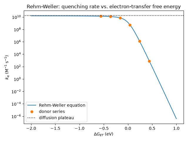
E_ox = 0.8 V: dG_ET = -0.56 eV, kq = 1.32e+10 1/(M s)
E_ox = 1.0 V: dG_ET = -0.36 eV, kq = 1.18e+10 1/(M s)
E_ox = 1.2 V: dG_ET = -0.16 eV, kq = 6.86e+09 1/(M s)
E_ox = 1.4 V: dG_ET = +0.04 eV, kq = 5.11e+08 1/(M s)
E_ox = 1.6 V: dG_ET = +0.24 eV, kq = 1.21e+06 1/(M s)
E_ox = 1.8 V: dG_ET = +0.44 eV, kq = 7.60e+02 1/(M s)

import matplotlib.pyplot as plt
import numpy as np

from chemistrykit.photochem import rehm_weller_free_energy, rehm_weller_quenching_rate

dG = np.linspace(-2.0, 1.0, 400)
kq = rehm_weller_quenching_rate(dG)

# A series of hypothetical donors quenching an excited acceptor with
# E00 = 2.9 eV and E_red = -1.6 V (vs. SCE).
E_ox = np.array([0.8, 1.0, 1.2, 1.4, 1.6, 1.8])
dG_pairs = np.array([rehm_weller_free_energy(E, -1.6, 2.9, work_term=-0.06) for E in E_ox])
rng = np.random.default_rng(7)
kq_meas = rehm_weller_quenching_rate(dG_pairs) * np.exp(rng.normal(0.0, 0.1, E_ox.size))

fig, ax = plt.subplots()
ax.semilogy(dG, kq, label="Rehm-Weller equation")
ax.semilogy(dG_pairs, kq_meas, "o", label="donor series")
ax.axhline(2.0e10 / 1.25, color="k", ls=":", label="diffusion plateau")
ax.set_xlabel(r"$\Delta G_{ET}$ (eV)")
ax.set_ylabel(r"$k_q$ (M$^{-1}$ s$^{-1}$)")
ax.set_title("Rehm-Weller: quenching rate vs. electron-transfer free energy")
ax.legend()
fig.tight_layout()

for E, g, k in zip(E_ox, dG_pairs, kq_meas):
    print(f"E_ox = {E:.1f} V: dG_ET = {g:+.2f} eV, kq = {k:.2e} 1/(M s)")

plt.show()