Bodenstein and Nernst: the H2 + Cl2 photochemical chain reaction

Bodenstein (1913) measured that one absorbed photon forms up to \(10^5\)-\(10^6\) HCl molecules in an illuminated H2/Cl2 mixture, apparently violating photochemical equivalence. Nernst (1918) explained it: the photon only splits one Cl2 into two Cl atoms, which then start a chain (Cl + H2 -> HCl + H, H + Cl2 -> HCl + Cl) that runs until two atoms recombine. hydrogen_chlorine_chain_network() integrates this mechanism, and chain_quantum_yield() gives the steady-state yield \(\Phi=2k_2[\mathrm{H_2}]/\sqrt{k_t I_{abs}}\). Rate constants are in arbitrary consistent units.

import matplotlib.pyplot as plt
import numpy as np

from chemistrykit.photochem import chain_quantum_yield, hydrogen_chlorine_chain_network

j, k2, k3, kt = 1.0e-4, 10.0, 100.0, 100.0
net = hydrogen_chlorine_chain_network(j, k2, k3, kt, H2_0=1.0, Cl2_0=1.0)
res = net.integrate((0.0, 30.0), dt=1e-3, method="rk4")

H2, Cl2, HCl = res.concentration("H2"), res.concentration("Cl2"), res.concentration("HCl")
I_abs = j * Cl2  # photons absorbed per unit volume per unit time
phi_numeric = np.gradient(HCl, res.t) / I_abs
phi_steady = chain_quantum_yield(k2, kt, H2, I_abs)

fig, ax = plt.subplots()
ax.plot(res.t, phi_numeric, label="integrated mechanism")
ax.plot(res.t, phi_steady, "k--", label=r"steady state $2k_2[H_2]/\sqrt{k_t I_{abs}}$")
ax.axhline(1.0, color="r", ls=":", label=r"Stark-Einstein $\Phi=1$")
ax.set_yscale("log")
ax.set_xlabel("Time")
ax.set_ylabel(r"HCl molecules per photon absorbed, $\Phi$")
ax.set_title("H$_2$ + Cl$_2$ chain: quantum yield far above 1")
ax.legend()
fig.tight_layout()
print(f"Quantum yield after the induction period: {phi_numeric[-1]:.0f} (steady-state formula {phi_steady[-1]:.0f})")

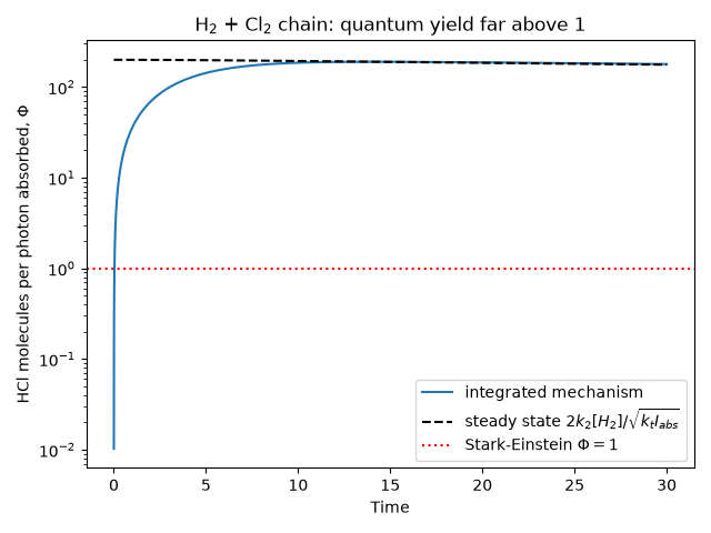
Quantum yield after the induction period: 179 (steady-state formula 177)

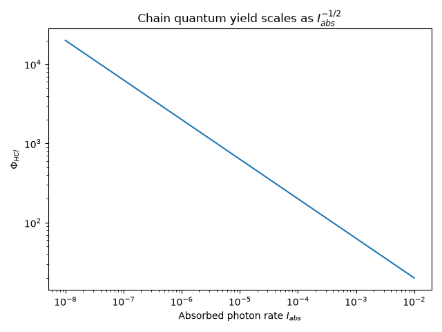
Chain length grows as the light gets weaker: fewer atoms means slower radical-radical termination, so each chain runs longer.

I = np.logspace(-8, -2, 50)
fig2, ax2 = plt.subplots()
ax2.loglog(I, chain_quantum_yield(k2, kt, 1.0, I))
ax2.set_xlabel(r"Absorbed photon rate $I_{abs}$")
ax2.set_ylabel(r"$\Phi_{HCl}$")
ax2.set_title(r"Chain quantum yield scales as $I_{abs}^{-1/2}$")
fig2.tight_layout()

plt.show()