Rayleigh-Schrodinger perturbation theory vs. exact diagonalization for the quartic oscillator

Schrodinger’s third 1926 paper introduced his perturbation theory; here it is applied to a harmonic oscillator with an added quartic term. Checks quartic_perturbation_first_order_correction()’s first-order Rayleigh-Schrodinger estimate against exact numerical diagonalization of the full anharmonic Hamiltonian (anharmonic_energy_levels(), built in a truncated harmonic-oscillator basis via position_operator_matrix()), and confirms that a cubic perturbation gives exactly zero first-order correction by parity.

import matplotlib.pyplot as plt
import numpy as np

from chemistrykit.constants import HBAR
from chemistrykit.quantum.systems.perturbation import (
    anharmonic_energy_levels,
    cubic_perturbation_first_order_correction,
    quartic_perturbation_first_order_correction,
)

mass, omega = 1.6e-27, 1.0e14

print("Cubic perturbation, first-order correction (always exactly zero by parity):")
for n in range(4):
    print(f"  n={n}: {cubic_perturbation_first_order_correction(n)}")

Cubic perturbation, first-order correction (always exactly zero by parity):
  n=0: 0.0
  n=1: 0.0
  n=2: 0.0
  n=3: 0.0

For a weak quartic perturbation, the first-order perturbative estimate should closely match the exact (numerically diagonalized) ground-state energy:

b_weak = 1.0e18
E0_harmonic = 0.5 * HBAR * omega
E0_perturbative = E0_harmonic + quartic_perturbation_first_order_correction(0, mass, omega, b_weak)
E0_exact = anharmonic_energy_levels(n_basis=40, mass=mass, omega=omega, b=b_weak, n_levels=1)[0]
print(f"\nWeak coupling (b = {b_weak:.1e} J/m^4):")
print(f"  harmonic E0:      {E0_harmonic:.6e} J")
print(f"  perturbative E0:  {E0_perturbative:.6e} J")
print(f"  exact E0:         {E0_exact:.6e} J")
print(f"  relative error:   {abs(E0_exact - E0_perturbative) / abs(E0_perturbative):.2e}")

Weak coupling (b = 1.0e+18 J/m^4):
  harmonic E0:      5.272859e-21 J
  perturbative E0:  5.273185e-21 J
  exact E0:         5.273185e-21 J
  relative error:   8.91e-09

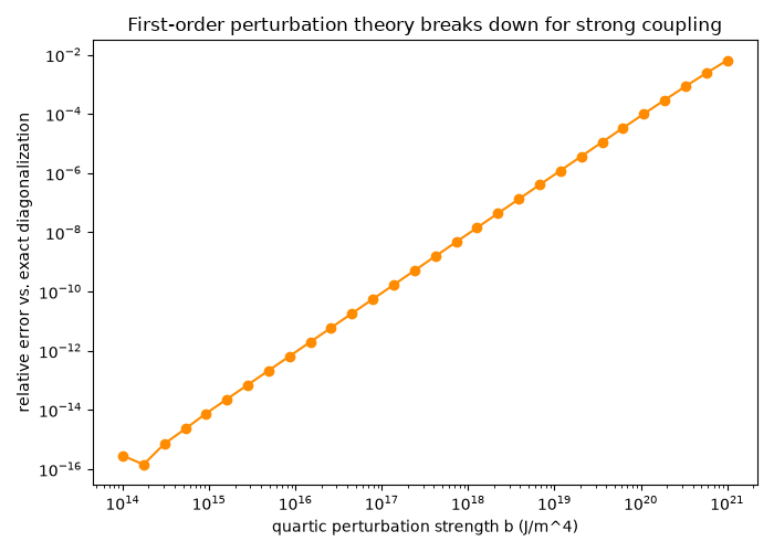
Perturbation theory degrades as the coupling strengthens – scanning b shows the relative error growing once the quartic term is no longer a small correction to the harmonic Hamiltonian:

b_values = np.logspace(14, 21, 30)
relative_errors = []
for b in b_values:
    E0_pert = E0_harmonic + quartic_perturbation_first_order_correction(0, mass, omega, b)
    E0_ex = anharmonic_energy_levels(n_basis=40, mass=mass, omega=omega, b=b, n_levels=1)[0]
    relative_errors.append(abs(E0_ex - E0_pert) / abs(E0_pert))

fig, ax = plt.subplots(figsize=(7, 5))
ax.loglog(b_values, relative_errors, "o-", color="darkorange")
ax.set_xlabel("quartic perturbation strength b (J/m^4)")
ax.set_ylabel("relative error vs. exact diagonalization")
ax.set_title("First-order perturbation theory breaks down for strong coupling")
fig.tight_layout()

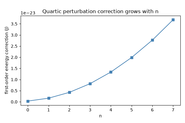
The perturbative correction itself grows with the vibrational quantum number n – higher states are more delocalized and probe the quartic term’s steep walls more strongly:

n_values = np.arange(0, 8)
corrections = [quartic_perturbation_first_order_correction(n, mass, omega, b_weak) for n in n_values]

fig2, ax2 = plt.subplots(figsize=(6, 4))
ax2.plot(n_values, corrections, "s-", color="steelblue")
ax2.set_xlabel("n")
ax2.set_ylabel("first-order energy correction (J)")
ax2.set_title("Quartic perturbation correction grows with n")
fig2.tight_layout()

plt.show()