Breakthroughs in Information Theory#
“The fundamental problem of communication is that of reproducing at one point either exactly or approximately a message selected at another point.” – Claude E. Shannon, 1948
Information theory is unusual among mathematical subjects in having a
birth certificate: Claude Shannon’s 1948 paper “A Mathematical Theory of
Communication,” which defined entropy, proved what compression and
error correction can and cannot achieve, and left the next fifty years
of engineers to find codes that live up to its promises. This
chronology traces the ideas behind
mathematicskit.information_theory, from Hartley’s logarithm and
Shannon’s theorems to Huffman’s optimal code, Hamming’s and Gallager’s
error-correcting codes, and the universal compressors of Elias, Ziv and
Lempel.
1928 – Hartley’s Measure of Information#
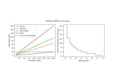
Ralph Hartley, an engineer at Bell Labs, set out in 1928 to measure information without reference to its meaning. A sender who makes \(L\) successive selections from an alphabet of \(n\) symbols picks one of \(n^L\) possible messages, and Hartley took the logarithm, \(H_0 = L\log n\), so that the information in a message grows in proportion to its length. Building on Harry Nyquist’s 1924 study of telegraph speed, he concluded that the information a line can carry is proportional to its bandwidth and to the time it is used. His measure treats all messages as equally likely, which is the gap Shannon filled twenty years later; the unit of \(\log_{10}\), the hartley, still carries his name.
Implementation: mathematicskit.information_theory.systems.entropy.hartley_information()
computes \(L\log n\) in any base, and the tests check that it equals
the Shannon entropy of the uniform distribution.
References: R. V. L. Hartley, “Transmission of Information,” Bell System Technical Journal 7(3) (1928), 535-563.
1948 – Shannon Entropy#
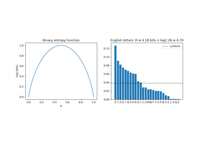
Claude Shannon’s 1948 paper replaced Hartley’s count of messages with an average over their probabilities. He asked for a measure of uncertainty that is continuous in the probabilities, increasing in the number of equally likely outcomes, and additive over successive choices, and proved that only one function qualifies: \(H = -\sum_i p_i \log p_i\). With base-2 logarithms it is counted in bits, a word Shannon credited to John Tukey. The name came, according to a story Shannon told later, from John von Neumann, who pointed out the formula’s resemblance to entropy in statistical mechanics. Shannon applied it to English and estimated the entropy of its letters, which is well below the \(\log_2 26\) bits a uniform alphabet would carry.
Implementation: mathematicskit.information_theory.systems.entropy.entropy()
wraps scipy.stats.entropy(), and
binary_entropy()
gives \(h(p)\) with scipy.special.entr(). The tests check the
bounds \(0 \le H \le \log_2 n\) and the change of base.
References: C. E. Shannon, “A Mathematical Theory of Communication,” Bell System Technical Journal 27 (1948), 379-423 and 623-656.
1948 – Mutual Information#
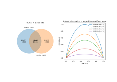
To measure what a noisy channel delivers, Shannon subtracted the uncertainty that remains about the input \(X\) once the output \(Y\) is seen: the rate of transmission \(I(X;Y) = H(X) - H(X\mid Y)\), later named the mutual information. It is symmetric in \(X\) and \(Y\), never negative, and zero exactly when the two are independent. Together with the chain rule \(H(X,Y) = H(X) + H(Y\mid X)\), it fits into a diagram of two overlapping circles whose overlap is the shared information. Its maximum over input distributions is the channel capacity.
Implementation: mathematicskit.information_theory.systems.entropy.mutual_information(),
joint_entropy()
and conditional_entropy()
work from a joint probability table, and
plot_information_diagram()
draws the diagram. The tests check the chain rule, the symmetry, and
that \(I(X;Y)\) equals the divergence of the joint distribution from
the product of its marginals.
References: Shannon (1948), Part II; T. M. Cover and J. A. Thomas, Elements of Information Theory, 2nd ed. (Hoboken: Wiley, 2006), Ch. 2.
1948 – The Source Coding Theorem and the Typical Set#
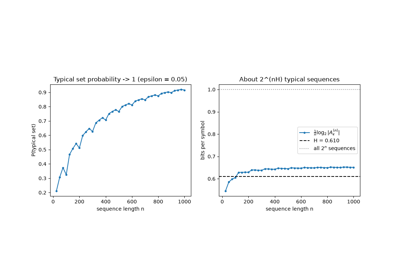
Shannon showed that entropy is the limit of lossless compression. For a long sequence of \(n\) independent symbols, \(-\tfrac1n\log_2 p(x^n)\) is almost always close to \(H\), so the sequences split into a “typical” set of about \(2^{nH}\) nearly equally likely members, which carries almost all the probability, and the rest. Indexing the typical set takes about \(nH\) bits, and no code can use fewer on average. Brockway McMillan extended this asymptotic equipartition property to stationary ergodic sources in 1953, and Leo Breiman strengthened it to almost-sure convergence in 1957.
Implementation: mathematicskit.information_theory.systems.source_coding.typical_set()
computes the size and probability of the typical set exactly, summing
over symbol counts with multinomial coefficients. The tests compare it
with brute-force enumeration and check the bounds
\((1-\varepsilon)2^{n(H-\varepsilon)} \le |A_\varepsilon^{(n)}| \le 2^{n(H+\varepsilon)}\).
References: Shannon (1948), Theorems 3 and 9; B. McMillan, “The Basic Theorems of Information Theory,” Annals of Mathematical Statistics 24(2) (1953), 196-219.
Shannon’s source coding theorem: the typical set (1948)
1948 – Capacity of the Binary Symmetric Channel#
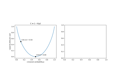
The simplest noisy channel flips each transmitted bit independently with probability \(p\). Shannon worked through it as his first example: at 1000 bits per second with \(p = 0.01\), the rate of transmission is not 990 bits per second, as subtracting the errors would suggest, but \(1000\,(1 - h(0.01)) \approx 919\), since the receiver does not know which bits are wrong. The capacity \(C = 1 - h(p)\), reached by a uniform input, falls to zero at \(p = 1/2\), where the output is independent of the input.
Implementation: mathematicskit.information_theory.systems.channels.bsc_capacity()
evaluates \(1 - h(p)\), and
bsc_transmit()
simulates the channel. The tests check the symmetry
\(C(p) = C(1-p)\) and that the mutual information of a uniform
input equals the capacity.
References: Shannon (1948), Section 13.
1948 – The Noisy-Channel Coding Theorem#
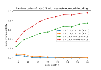
Shannon’s most surprising result was that noise limits the rate of communication, not its reliability: every rate below the capacity \(C\) can be sent with an error probability as small as desired, and no rate above it can. His proof did not construct a good code. It averaged over codes whose \(2^{nR}\) codewords are drawn at random, showed that the average error probability tends to zero with the block length when \(R < C\), and concluded that some code must do at least as well. Engineers took half a century to find practical codes that come close, through turbo codes (1993) and the rediscovery of LDPC codes.
Implementation: mathematicskit.information_theory.systems.channels.random_code_error_rate()
reproduces the random-coding experiment on a binary symmetric channel
with nearest-codeword decoding. The tests check that the error rate
falls with the block length below capacity and exceeds 0.8 above it.
References: Shannon (1948), Theorem 11; R. G. Gallager, Information Theory and Reliable Communication (New York: Wiley, 1968), Ch. 5.
1948-1949 – Shannon-Fano Coding#
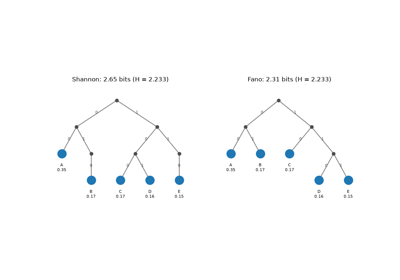
The first codes built on Shannon’s theory came from Shannon himself and
from Robert Fano at MIT. Shannon gave the \(i\)-th most likely
symbol \(\lceil -\log_2 p_i\rceil\) bits, read from the binary
expansion of the cumulative probability of the more likely symbols.
Fano sorted the symbols and split them recursively into two groups of
nearly equal total probability, labelling the groups 0 and 1.
Both methods give a prefix code whose average length is within one bit
of the entropy, which is enough to prove the source coding theorem, but
neither is always optimal.
Implementation: mathematicskit.information_theory.systems.source_coding.shannon_fano_code()
implements both constructions (method="shannon" and
method="fano"), returning a
PrefixCode. The
tests check the bound \(H \le \bar L < H + 1\) and Shannon’s
codeword lengths.
References: Shannon (1948), Section 9; R. M. Fano, The Transmission of Information, Technical Report 65, MIT Research Laboratory of Electronics (1949).
1949 – The Shannon-Hartley Theorem#
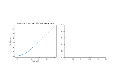
In “Communication in the Presence of Noise,” Shannon turned to continuous signals. Using the sampling theorem to represent a signal of bandwidth \(B\) by \(2B\) samples per second, and a geometric argument about packing spheres in many dimensions, he proved that a channel with average power \(S\) and white Gaussian noise of power \(N\) carries at most \(C = B\log_2(1 + S/N)\) bits per second. Capacity grows only logarithmically with power. Per bit, it sets a floor: no code communicates reliably below \(E_b/N_0 = \ln 2\), or \(-1.59\) dB, the Shannon limit that modern codes are measured against.
Implementation: mathematicskit.information_theory.systems.channels.awgn_capacity()
evaluates the formula, and
minimum_ebn0()
gives the smallest \(E_b/N_0\) for a spectral efficiency. The tests
check the limit \(\ln 2\).
References: C. E. Shannon, “Communication in the Presence of Noise,” Proceedings of the IRE 37(1) (1949), 10-21.
1949, 1956 – The Kraft-McMillan Inequality#
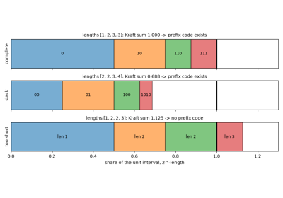
Leon Kraft’s 1949 master’s thesis at MIT answered which codeword lengths a prefix code can have: lengths \(\ell_i\) are possible if and only if \(\sum_i 2^{-\ell_i} \le 1\). Each codeword of length \(\ell\) claims a \(2^{-\ell}\) share of the binary tree, and prefix-freeness forbids the shares to overlap. In 1956 Brockway McMillan proved that the same inequality holds for every uniquely decodable code, so nothing is lost by insisting on prefix codes. The inequality turns code design into the choice of lengths, and with \(\ell_i \approx -\log_2 p_i\) it gives the entropy bound.
Implementation: mathematicskit.information_theory.systems.source_coding.kraft_sum()
evaluates the sum, and
canonical_code()
constructs a prefix code with any admissible lengths. The tests check
the construction and the rejection of lengths whose sum exceeds 1.
References: L. G. Kraft, A Device for Quantizing, Grouping, and Coding Amplitude-Modulated Pulses, MS thesis, MIT (1949); B. McMillan, “Two Inequalities Implied by Unique Decipherability,” IRE Transactions on Information Theory 2(4) (1956), 115-116.
1950 – Hamming Codes#
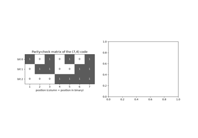
Richard Hamming ran his programs over weekends on Bell Labs’ relay computers, which stopped a job whenever they detected an error. His frustration led him to codes that correct errors as well as detect them. The (7,4) Hamming code adds three parity bits to four data bits; each parity bit checks the positions whose binary expansion contains its own bit, so the pattern of failed checks, the syndrome, spells out the position of a single error. Hamming also introduced the distance between binary words that bears his name and showed that a minimum distance of \(2t+1\) corrects \(t\) errors.
Implementation: mathematicskit.information_theory.systems.channel_codes.hamming_encode()
and hamming_decode()
implement the \((2^r-1, 2^r-r-1)\) codes with syndrome decoding.
The tests check that every single error is corrected and that the
(7,4) code has minimum distance 3.
References: R. W. Hamming, “Error Detecting and Error Correcting Codes,” Bell System Technical Journal 29(2) (1950), 147-160.
1951 – The Kullback-Leibler Divergence#
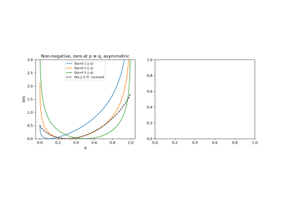
Solomon Kullback and Richard Leibler, cryptanalysts at the US National Security Agency, defined the mean information per observation for discriminating between two hypotheses, \(D(p\,\|\,q) = \sum p\log(p/q)\). It is never negative, by Gibbs’ inequality, and vanishes only when \(p = q\), but it is not symmetric and so not a distance. In coding terms it is the number of extra bits per symbol paid for compressing a \(p\)-source with a code designed for \(q\). It became the common currency of information theory, statistics and machine learning: mutual information, likelihood ratio tests and variational inference are all built on it.
Implementation: mathematicskit.information_theory.systems.entropy.kl_divergence()
wraps scipy.stats.entropy() with two arguments. The tests check
Gibbs’ inequality on random distributions, the asymmetry, and the
infinite value when \(q\) misses part of the support of \(p\).
References: S. Kullback and R. A. Leibler, “On Information and Sufficiency,” Annals of Mathematical Statistics 22(1) (1951), 79-86.
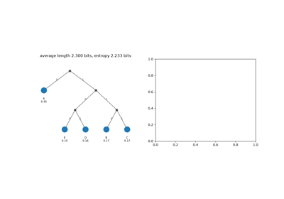
1952 – Huffman Coding#
David Huffman was a graduate student in Robert Fano’s information theory
class at MIT in 1951 when Fano offered the class a choice between a
final exam and a term paper on finding the most efficient binary code,
a problem Fano and Shannon had not solved. Huffman found the answer by
building the code tree from the bottom up instead of the top down:
merge the two least likely symbols into one node, and repeat. The
result is optimal among all prefix codes, and Huffman codes are still
part of JPEG, MP3 and the DEFLATE format used by zip and PNG.
Implementation: mathematicskit.information_theory.systems.source_coding.huffman_code()
builds the code with a priority queue (heapq), and
plot_code_tree()
draws its tree. The tests check optimality against a brute-force
search over all admissible lengths, and that no Shannon-Fano code is
shorter.
References: D. A. Huffman, “A Method for the Construction of Minimum-Redundancy Codes,” Proceedings of the IRE 40(9) (1952), 1098-1101.
1955 – Convolutional Codes#
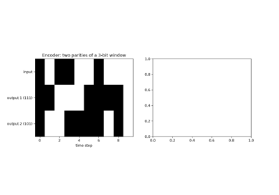
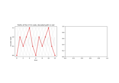
Peter Elias proposed encoding a stream of bits continuously rather than in blocks. A convolutional encoder slides a short window, the constraint length \(K\), along the input, and outputs several parities of each window position, so each input bit influences several consecutive outputs. Elias showed that such codes, with random generators, achieve the same error exponents as random block codes. In the same paper he introduced the binary erasure channel, whose capacity is \(1 - \varepsilon\). With Viterbi decoding, convolutional codes became the workhorse of deep-space and mobile communication.
Implementation: mathematicskit.information_theory.systems.channel_codes.convolutional_encode()
implements a feed-forward encoder with arbitrary generators (default
\((7, 5)_8\), \(K=3\)), and
bec_capacity()
gives the erasure channel’s capacity. The tests check linearity and the
free distance of 5.
References: P. Elias, “Coding for Noisy Channels,” IRE Convention Record 3(4) (1955), 37-46.
1959 – Rate-Distortion Theory#
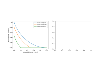
Lossless compression cannot go below the entropy, and a continuous source has no finite lossless description at all. Shannon’s 1959 paper asked how few bits suffice when the reconstruction may differ from the source by an average distortion \(D\). The answer is the rate-distortion function \(R(D)\), the least mutual information between source and reconstruction among all reconstructions within distortion \(D\). For a fair coin with Hamming distortion it is \(1 - h(D)\); for a Gaussian source with squared error it is \(\tfrac12\log_2(\sigma^2/D)\), so each extra bit divides the error by four. It is the theoretical basis of lossy compression of audio, images and video.
Implementation: mathematicskit.information_theory.systems.channels.rate_distortion_binary()
and rate_distortion_gaussian()
evaluate the two closed forms. The tests check the endpoints and the
half bit gained per halving of the Gaussian distortion.
References: C. E. Shannon, “Coding Theorems for a Discrete Source with a Fidelity Criterion,” IRE National Convention Record 7(4) (1959), 142-163.
1962-1963 – Gallager’s Low-Density Parity-Check Codes#
Robert Gallager’s doctoral thesis at MIT defined codes by a random parity-check matrix with only a few ones in each row and column, and decoded them iteratively: each bit looks at the checks it takes part in and flips if most of them fail, and the process repeats. He proved that such codes have good distance and that iterative decoding corrects many errors, but the computers of the 1960s could not run the decoders at useful block lengths, and the codes were largely forgotten. David MacKay and Radford Neal rediscovered them in 1996, showing that with belief-propagation decoding they come within a fraction of a decibel of capacity. LDPC codes are now part of Wi-Fi, 5G and digital television standards.
Implementation: mathematicskit.information_theory.systems.channel_codes.gallager_ldpc_matrix()
builds Gallager’s regular random matrices, and
bit_flip_decode()
runs the hard-decision bit-flipping decoder, returning a
BitFlipResult.
The tests check the row and column weights and that sparse errors are
corrected.
References: R. G. Gallager, “Low-Density Parity-Check Codes,” IRE Transactions on Information Theory 8(1) (1962), 21-28; R. G. Gallager, Low-Density Parity-Check Codes (Cambridge, MA: MIT Press, 1963); D. J. C. MacKay and R. M. Neal, “Near Shannon Limit Performance of Low Density Parity Check Codes,” Electronics Letters 32(18) (1996), 1645.
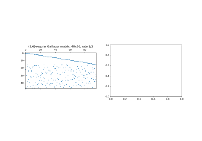
Gallager’s low-density parity-check codes (1962-1963)
1967 – The Viterbi Algorithm#
Andrew Viterbi introduced his algorithm as a tool for bounding the error probability of convolutional codes. Decoding by exhaustive search costs time exponential in the message length, but the encoder has only \(2^{K-1}\) states, and among all paths that reach a state at a given time only the one closest to the received sequence can be part of the best overall path. Keeping one survivor per state makes maximum-likelihood decoding linear in the message length. David Forney showed in 1973 that it is exactly dynamic programming on the trellis of states. The algorithm decoded the Voyager and Galileo missions, mobile phones, and later speech recognition with hidden Markov models; Viterbi went on to co-found Qualcomm.
Implementation: mathematicskit.information_theory.systems.channel_codes.viterbi_decode()
performs hard-decision Viterbi decoding of a terminated convolutional
code. The tests check that every pattern of two errors in a short block
is corrected, and that the decoded bit error rate on a binary symmetric
channel is well below the uncoded one.
References: A. J. Viterbi, “Error Bounds for Convolutional Codes and an Asymptotically Optimum Decoding Algorithm,” IEEE Transactions on Information Theory 13(2) (1967), 260-269; G. D. Forney, “The Viterbi Algorithm,” Proceedings of the IEEE 61(3) (1973), 268-278.
1972 – The Blahut-Arimoto Algorithm#
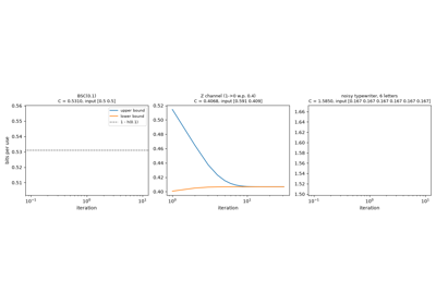
The capacity of a channel is a maximum of mutual information over input distributions, and only symmetric channels give it in closed form. Richard Blahut and Suguru Arimoto independently published, in the same volume of the IEEE Transactions on Information Theory, an alternating algorithm that computes it for any discrete memoryless channel. Each step reweights the input distribution by the exponential of each input’s divergence from the current output distribution. Every iteration brackets the capacity between a lower and an upper bound, which converge, so the algorithm certifies its own accuracy. Blahut’s paper also gave the analogous algorithm for the rate-distortion function.
Implementation: mathematicskit.information_theory.systems.channels.blahut_arimoto()
returns a ChannelCapacityResult
with the capacity, the optimal input distribution, and both bounds at
every iteration. The tests check it against the closed forms for the
binary symmetric, binary erasure and Z channels.
References: R. E. Blahut, “Computation of Channel Capacity and Rate-Distortion Functions,” IEEE Transactions on Information Theory 18(4) (1972), 460-473; S. Arimoto, “An Algorithm for Computing the Capacity of Arbitrary Discrete Memoryless Channels,” IEEE Transactions on Information Theory 18(1) (1972), 14-20.
1975 – Elias’ Universal Codes for the Integers#
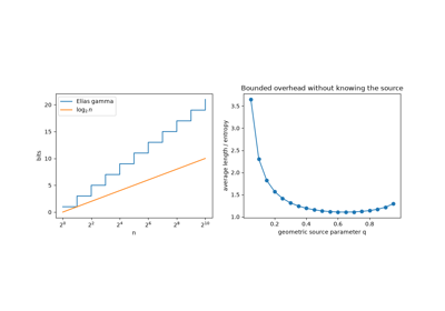
Huffman’s code needs the source probabilities in advance. Peter Elias asked how to code positive integers whose distribution is unknown, needing only that larger values are no more likely than smaller ones. His gamma code writes \(\lfloor\log_2 n\rfloor\) zeros followed by \(n\) in binary, so the zeros announce how many digits follow. It is a prefix code for all positive integers at once, with length \(2\lfloor\log_2 n\rfloor + 1\), and on every decreasing distribution its average length is within a constant factor of the entropy, a property Elias called universality. His delta and omega codes refine the same idea, and such codes are still used to compress the integer lists in search-engine indexes.
Implementation: mathematicskit.information_theory.systems.source_coding.elias_gamma_encode()
and elias_gamma_decode()
encode single integers and decode concatenated streams. The tests check
the round trip and the codeword lengths.
References: P. Elias, “Universal Codeword Sets and Representations of the Integers,” IEEE Transactions on Information Theory 21(2) (1975), 194-203.
1976 – Arithmetic Coding#
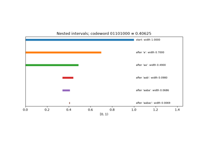
Huffman codes waste up to a bit per symbol, which is costly when one symbol is very likely. Jorma Rissanen at IBM and Richard Pasco at Stanford independently showed in 1976 how to code an entire message as a single number. Each symbol narrows an interval in proportion to its probability, and the codeword is the shortest binary fraction inside the final interval, within two bits of \(-\log_2 p(\text{message})\). The idea, which had been sketched by Elias and others without a practical finite-precision form, became practical with the integer implementation of Ian Witten, Radford Neal and John Cleary (1987), and is now used in JPEG 2000 and H.264/H.265 video.
Implementation: mathematicskit.information_theory.systems.source_coding.arithmetic_encode(),
arithmetic_decode()
and arithmetic_intervals()
use exact rational arithmetic (fractions.Fraction), so the
interval narrowing is visible without the rescaling tricks practical
coders need. The tests check the round trip and the length bound.
References: J. Rissanen, “Generalized Kraft Inequality and Arithmetic Coding,” IBM Journal of Research and Development 20(3) (1976), 198-203; R. C. Pasco, Source Coding Algorithms for Fast Data Compression, PhD thesis, Stanford University (1976); I. H. Witten, R. M. Neal and J. G. Cleary, “Arithmetic Coding for Data Compression,” Communications of the ACM 30(6) (1987), 520-540.
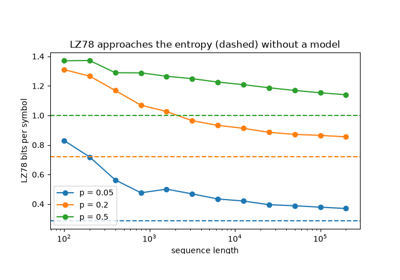
1977-1978 – Lempel-Ziv Compression#
Abraham Lempel and Jacob Ziv, at the Technion, designed compressors
that need no model of the source at all. Their 1977 algorithm (LZ77)
replaces repeated strings by pointers back into a sliding window; the
1978 algorithm (LZ78) parses the input into phrases, each the longest
earlier phrase plus one new symbol, and sends a phrase index and a
symbol. Ziv and Lempel proved that, for any stationary ergodic source,
the compressed length per symbol approaches the entropy rate, so a
single algorithm is asymptotically optimal for every such source.
Terry Welch’s 1984 variant, LZW, was used in Unix compress and GIF
images, and LZ77 lives on in DEFLATE, the format of zip, gzip
and PNG.
Implementation: mathematicskit.information_theory.systems.source_coding.lz78_encode()
and lz78_decode()
implement the LZ78 parsing, and
lz78_compressed_bits()
counts the bits of the encoded phrases. The tests check the round trip
and the compression of a low-entropy source.
References: J. Ziv and A. Lempel, “A Universal Algorithm for Sequential Data Compression,” IEEE Transactions on Information Theory 23(3) (1977), 337-343; J. Ziv and A. Lempel, “Compression of Individual Sequences via Variable-Rate Coding,” IEEE Transactions on Information Theory 24(5) (1978), 530-536.