Breakthroughs in Dynamical Systems#

mathematicskit.ode_dynamics hub · History · Examples · API reference

“It may happen that small differences in the initial conditions produce very great ones in the final phenomena.” – Henri Poincaré, Science et méthode, 1908

A dynamical system’s qualitative behavior – does it settle down, spiral in, oscillate forever, or wander chaotically? – can often be understood without solving its equations exactly. This chronology traces the ideas behind mathematicskit.ode_dynamics: the classification of linear flows near a fixed point, the discovery of self-sustained oscillation, and the slow, then sudden, realization that simple deterministic systems can behave unpredictably. Interleaved with these are the numerical methods behind mathematicskit.integrators that compute every trajectory: Euler’s, Adams-Bashforth and Runge-Kutta methods, symplectic and adaptive integrators, the discovery of stiffness and the implicit methods that tame it, and collocation for boundary-value problems.

1768 – Euler’s Method #

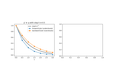
In the first volume of his Institutiones calculi integralis, Leonhard Euler proposed approximating a solution of \(y' = f(t, y)\) by following its tangent line for a short step \(h\):

\[y_{n+1} = y_n + h\,f(t_n, y_n).\]

Each step makes an error of order \(h^2\). Over the \(1/h\) steps needed to reach a fixed time these add up to a global error of order \(h\), so halving the step halves the error. Evaluating the slope at the end of the step instead, \(y_{n+1} = y_n + h f(t_{n+1}, y_{n+1})\), gives the implicit (backward) Euler method. It is just as accurate, but it requires solving an equation for \(y_{n+1}\) at every step, a cost that pays off for stiff equations (see Curtiss and Hirschfelder and Dahlquist, below). Cauchy later used Euler’s polygons to prove that solutions exist.

Implementation: mathematicskit.integrators.euler_integrate() implements the explicit method, and implicit_euler_integrate() implements backward Euler, solving for each step with Newton’s method and a finite-difference Jacobian. The tests check the closed forms \((1 - \lambda h)^n\) and \(y/(1 + \lambda h)\) on \(y' = -\lambda y\), and that for both methods the error ratio for halved \(h\) is 2.

References: L. Euler, Institutionum calculi integralis, vol. 1 (St. Petersburg, 1768).

Euler’s method: first-order convergence

Euler's method: first-order convergence

1838 – Verhulst’s Logistic Equation #

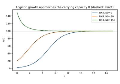
Thomas Malthus had argued that populations grow geometrically. Pierre-François Verhulst noted that resources are limited. He proposed that the per-capita growth rate should decline as the population approaches a ceiling, the carrying capacity \(K\):

\[\dot N = rN\left(1 - \frac{N}{K}\right), \qquad N(t) = \frac{K}{1 + \left(\frac{K - N_0}{N_0}\right)e^{-rt}}.\]

This was one of the first nonlinear differential equations used to model a real population, and one of the few that can be solved exactly. Its S-shaped “logistic” solution grows fastest at \(N = K/2\) and levels off at \(K\). The stable fixed point \(N = K\) and the unstable fixed point \(N = 0\) make it the standard first example of one-dimensional phase-line analysis.

Implementation: mathematicskit.ode_dynamics.systems.population.LogisticGrowth integrates the equation, and logistic_growth_solution() evaluates Verhulst’s closed form. The tests check that the two agree to about \(10^{-8}\).

References: P.-F. Verhulst, “Notice sur la loi que la population suit dans son accroissement,” Correspondance Mathématique et Physique 10 (1838), 113-121.

Verhulst’s logistic growth

Verhulst's logistic growth

1881-1886 – Poincaré’s Qualitative Theory of ODEs #

Henri Poincaré’s series of memoirs “Sur les courbes définies par une équation différentielle” founded a new way of studying differential equations. Instead of seeking a closed-form solution, he studied the qualitative structure of the flow directly in the phase plane. He classified fixed points as nodes, saddles, spirals (foci), or centers according to the eigenvalues of the linearized flow, the basis of the trace-determinant classification still taught today.

\[\tau = \operatorname{tr}(J), \qquad \Delta = \det(J), \qquad \lambda_{1,2} = \frac{\tau \pm \sqrt{\tau^2 - 4\Delta}}{2}\]

Implementation: mathematicskit.ode_dynamics.systems.stability.classify_fixed_point_2d() implements this \((\tau,\Delta)\)-plane classification, and Linear2D/ Nonlinear2D render the corresponding phase portraits.

References: H. Poincaré, “Sur les courbes définies par une équation différentielle,” Journal de Mathématiques Pures et Appliquées, four installments (1881-1886).

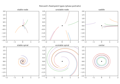
Poincaré’s classification of fixed points: nodes, saddles, spirals, centers

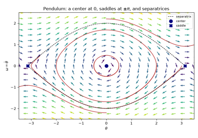
Poincaré's classification of fixed points: nodes, saddles, spirals, centers

Poincaré’s qualitative method: the pendulum’s phase portrait

Poincaré's qualitative method: the pendulum's phase portrait

1883 – Bashforth and Adams: Linear Multistep Methods #

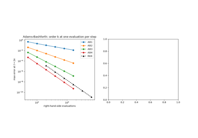
Francis Bashforth needed accurate profiles of liquid drops to test the theory of capillarity, and John Couch Adams, codiscoverer of Neptune, supplied the numerical method in their 1883 book. Every step of a one-step method computes fresh slopes and then discards them. Adams kept the last \(k\) of them, fitted a polynomial through them, and integrated it across the next step:

\[y_{n+1} = y_n + h \sum_{j=0}^{k-1} \beta_j f_{n-j}, \qquad \text{e.g.}\quad y_{n+1} = y_n + h\left(\tfrac32 f_n - \tfrac12 f_{n-1}\right).\]

The result has order \(k\) but needs only one new evaluation of \(f\) per step. Forest Ray Moulton added the implicit companion formulas in 1926 for ballistics tables, and Adams-Bashforth-Moulton predictor-corrector pairs were the standard ODE solvers of the early computer era. Reusing old information has a cost: the method needs \(k - 1\) starting values, and its stability region shrinks as the order grows, to a real interval of only \([-0.3, 0]\) for order 4.

Implementation: mathematicskit.integrators.adams_bashforth_integrate() implements orders 1 to 4, starting with RK4 steps, and adams_bashforth_boundary_locus() and is_absolutely_stable() compute the stability regions. The tests check that halving \(h\) divides the error by \(2^k\), that order 3 is exact for quadratic slopes, and that the regions’ real intervals are \([-2, 0]\), \([-1, 0]\), \([-6/11, 0]\) and \([-3/10, 0]\).

References: F. Bashforth and J. C. Adams, An Attempt to Test the Theories of Capillary Action by Comparing the Theoretical and Measured Forms of Drops of Fluid (Cambridge University Press, 1883); F. R. Moulton, New Methods in Exterior Ballistics (University of Chicago Press, 1926); E. Hairer, S. P. Nørsett, and G. Wanner, Solving Ordinary Differential Equations I, 2nd ed. (Springer, 1993), sec. III.1.

Bashforth and Adams: linear multistep methods

1892 – Lyapunov’s Direct Method #

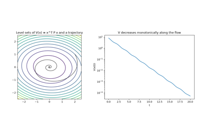
In his doctoral thesis The General Problem of the Stability of Motion, Aleksandr Lyapunov proved stability without solving the equations of motion. He generalized the idea of energy. Suppose a function \(V(x)\) is positive everywhere except at the equilibrium, where it is zero, and strictly decreases along every trajectory. Then every trajectory must slide down toward the equilibrium, which is therefore asymptotically stable. For a linear system \(\dot x = Ax\), the quadratic form \(V = x^T P x\) works exactly when \(P\) solves the Lyapunov equation

\[A^T P + P A = -Q, \qquad Q \succ 0,\]

and a positive-definite solution \(P\) exists if and only if every eigenvalue of \(A\) has negative real part. Lyapunov functions remain the main tool for proving the stability of nonlinear systems and of control systems.

Implementation: mathematicskit.ode_dynamics.systems.stability.lyapunov_quadratic_form() solves the Lyapunov equation with SciPy’s Bartels-Stewart solver and returns a LyapunovFunctionResult. The tests check the residual of the equation and confirm that \(V\) decreases monotonically along integrated trajectories.

References: A. M. Lyapunov, The General Problem of the Stability of Motion (Kharkov Mathematical Society, 1892; in Russian), English translation by A. T. Fuller, International Journal of Control 55(3) (1992), 531-773.

Lyapunov’s direct method

Lyapunov's direct method

1895-1901 – Runge, Heun, and Kutta: Runge-Kutta Methods #

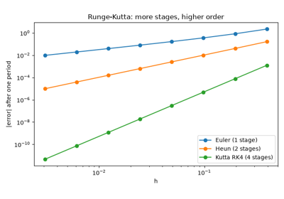
Carl Runge asked how to get the accuracy of a high-order Taylor series without differentiating \(f\). His answer was to evaluate the slope at several points inside each step and combine them. Karl Heun gave second- and third-order schemes, and Wilhelm Kutta derived the order conditions systematically, including the classical fourth-order method

\[k_1 = f(t_n, y_n),\quad k_2 = f(t_n + \tfrac h2, y_n + \tfrac h2 k_1),\quad k_3 = f(t_n + \tfrac h2, y_n + \tfrac h2 k_2),\quad k_4 = f(t_n + h, y_n + h k_3),\]

\[y_{n+1} = y_n + \tfrac h6 (k_1 + 2k_2 + 2k_3 + k_4).\]

Halving \(h\) divides the error by 16. “RK4” became the default integrator for well over half a century, and it is still the default in mathematicskit.ode_dynamics.

Implementation: mathematicskit.integrators.rk4_integrate() (Numba-compiled, reusing one compiled right-hand side across parameter values). The tests check it against the harmonic oscillator’s exact solution.

References: C. Runge, “Über die numerische Auflösung von Differentialgleichungen,” Mathematische Annalen 46 (1895), 167-178; K. Heun, “Neue Methoden zur approximativen Integration der Differentialgleichungen einer unabhängigen Veränderlichen,” Zeitschrift für Mathematik und Physik 45 (1900), 23-38; W. Kutta, “Beitrag zur näherungsweisen Integration totaler Differentialgleichungen,” Zeitschrift für Mathematik und Physik 46 (1901), 435-453.

Runge, Heun and Kutta: Runge-Kutta methods

1901 – Bendixson’s Negative Criterion #

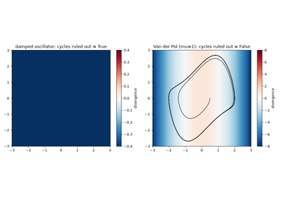
Ivar Bendixson’s long memoir in Acta Mathematica completed Poincaré’s picture of planar flows. Its best-known result is the Poincaré-Bendixson theorem: a bounded planar trajectory that avoids fixed points must approach a periodic orbit. The same memoir also gives a simple test for ruling periodic orbits out. If the divergence

\[\nabla\cdot F = \frac{\partial f}{\partial x} + \frac{\partial g}{\partial y}\]

of the vector field \(F = (f, g)\) does not change sign and is not identically zero on a simply connected region, that region contains no closed orbit. By Green’s theorem, the integral of the divergence over the region inside a closed orbit equals the flux across the orbit. That flux is zero, because the flow runs along the orbit and never across it.

Implementation: mathematicskit.ode_dynamics.systems.limit_cycles.bendixson_criterion() samples the divergence on a grid and returns a BendixsonResult. It rules out cycles for damped oscillators, but not for a linear center or for the Van der Pol field, whose divergence changes sign at \(|x| = 1\).

References: I. Bendixson, “Sur les courbes définies par des équations différentielles,” Acta Mathematica 24 (1901), 1-88.

Bendixson’s negative criterion

Bendixson's negative criterion

1907-1967 – Störmer, Verlet, and Symplectic Integration #

Carl Størmer computed the orbits of charged particles in the Earth’s magnetic field, to explain the aurora, with a simple scheme for \(\ddot q = F(q)\). Loup Verlet rediscovered it for molecular dynamics in 1967. In “velocity Verlet” (leapfrog) form it reads

\[v_{n+1/2} = v_n + \tfrac h2 F(q_n),\quad q_{n+1} = q_n + h\,v_{n+1/2},\quad v_{n+1} = v_{n+1/2} + \tfrac h2 F(q_{n+1}).\]

It is only second order, but it is time-reversible and symplectic: it preserves phase-space area exactly, and it exactly conserves a modified energy within \(O(h^2)\) of the true one. As a result its energy error stays bounded for exponentially long times, while a non-symplectic method, even a higher-order one like RK4, drifts steadily. This explanation came later, from backward error analysis in the 1990s, and it is why molecular-dynamics and celestial-mechanics codes still use leapfrog.

Implementation: mathematicskit.integrators.leapfrog_integrate() (alias velocity_verlet_integrate). The tests check that the harmonic-oscillator energy is conserved to \(10^{-4}\) over 20,000 steps.

References: C. Størmer, “Sur les trajectoires des corpuscules électrisés dans l’espace sous l’action du magnétisme terrestre,” Archives des Sciences Physiques et Naturelles 24 (1907); L. Verlet, “Computer ‘Experiments’ on Classical Fluids. I,” Physical Review 159 (1967), 98-103; E. Hairer, C. Lubich, and G. Wanner, “Geometric Numerical Integration Illustrated by the Störmer-Verlet Method,” Acta Numerica 12 (2003), 399-450.

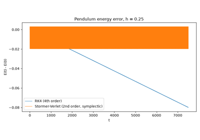
Stormer-Verlet: bounded energy error over long times

1918-1961 – Duffing, Ueda, and the Stroboscopic Poincaré Section #

Georg Duffing’s 1918 monograph analyzed the forced, damped oscillator with a cubic nonlinearity that now bears his name. Its chaotic regime was first revealed by Yoshisuke Ueda’s numerical experiments in 1961, which were published more widely from 1970 onward. Ueda used a tool that Henri Poincaré had introduced for the three-body problem seven decades earlier: sample the state once per drive period instead of plotting the continuous trajectory. A hopelessly tangled orbit becomes a scatter of points whose pattern is easy to read – a few dots for periodic motion, a structureless or fractal-looking cloud for chaos.

Implementation: mathematicskit.ode_dynamics.systems.poincare.DuffingOscillator integrates Duffing’s equation, and stroboscopic_poincare_section() implements this once-per-period sampling.

References: G. Duffing, Erzwungene Schwingungen bei veränderlicher Eigenfrequenz und ihre technische Bedeutung (Braunschweig: Vieweg, 1918); Y. Ueda, “Randomly Transitional Phenomena in the System Governed by Duffing’s Equation,” Journal of Statistical Physics 20(2) (1979), 181-196 (a widely cited later account of the phenomenon Ueda’s simulations first found in 1961).

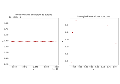
Poincare sections of the driven Duffing oscillator

1920-1926 – Lotka, Volterra, and Predator-Prey Cycles #

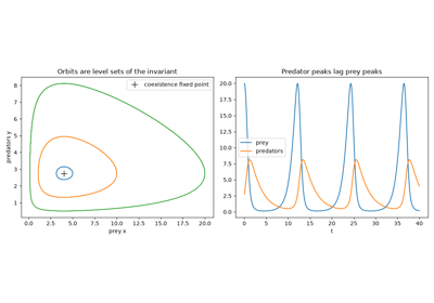
Alfred Lotka found sustained oscillations in a model of coupled chemical and biological processes. Independently, Vito Volterra was asked by the marine biologist Umberto D’Ancona why the share of predatory fish in Adriatic catches rose during the First World War, when fishing was reduced. Both arrived at the same model:

\[\dot x = \alpha x - \beta xy, \qquad \dot y = \delta xy - \gamma y.\]

The prey \(x\) and predators \(y\) cycle out of phase, with predator peaks lagging prey peaks. Volterra showed that the quantity \(V = \delta x - \gamma\ln x + \beta y - \alpha\ln y\) stays constant along every trajectory. The orbits are therefore closed curves around the coexistence point \((\gamma/\delta, \alpha/\beta)\), and small oscillations have period \(2\pi/\sqrt{\alpha\gamma}\).

Implementation: mathematicskit.ode_dynamics.systems.population.LotkaVolterra integrates the system, and lotka_volterra_invariant() evaluates Volterra’s conserved quantity. The tests check that it is conserved to \(10^{-8}\), and that the small-oscillation period matches the linearized value.

References: A. J. Lotka, “Analytical Note on Certain Rhythmic Relations in Organic Systems,” Proceedings of the National Academy of Sciences 6(7) (1920), 410-415; V. Volterra, “Fluctuations in the Abundance of a Species considered Mathematically,” Nature 118 (1926), 558-560.

Lotka-Volterra predator-prey cycles

1926 – van der Pol and the Relaxation Oscillator #

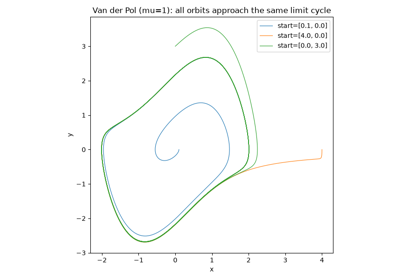
Balthasar van der Pol studied the vacuum-tube circuits of early radio. He found that a particular nonlinear damping term – one that removes energy from large oscillations but adds energy to small ones – produces a self-sustained oscillation of fixed amplitude and shape, whatever the initial condition. Such an isolated periodic orbit is called a limit cycle. It is the standard example of the conclusion of the Poincaré-Bendixson theorem: a planar trajectory that stays in a bounded region containing no fixed point must approach a periodic orbit.

\[\ddot x - \mu(1-x^2)\dot x + x = 0\]

Implementation: mathematicskit.ode_dynamics.systems.limit_cycles.VanDerPolOscillator integrates this equation, and estimate_limit_cycle_amplitude() measures the amplitude the system settles into from any starting point.

References: B. van der Pol, “On Relaxation-Oscillations,” The London, Edinburgh, and Dublin Philosophical Magazine and Journal of Science, Series 7, 2(11) (1926), 978-992.

The Van der Pol limit cycle

1927 – Kermack and McKendrick’s Epidemic Threshold #

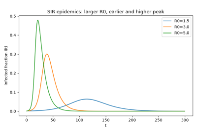
William Kermack and Anderson McKendrick divided a population into susceptible, infected, and removed classes. They showed that an epidemic can burn out long before everyone has been infected:

\[\dot S = -\beta SI, \qquad \dot I = \beta SI - \gamma I, \qquad \dot R = \gamma I.\]

An outbreak grows only when the basic reproduction number \(R_0 = \beta/\gamma\), multiplied by the susceptible fraction, exceeds one. This threshold theorem is the mathematical basis of herd immunity. The equations also give exact answers without solving for \(S(t)\). Infections peak when \(S = 1/R_0\), and the fraction never infected, \(S_\infty\), solves the final-size equation \(\ln(S_0/S_\infty) = R_0(S_0 + I_0 - S_\infty)\).

Implementation: mathematicskit.ode_dynamics.systems.epidemics.SIRModel integrates the model, and sir_final_size() and sir_peak_infected() evaluate the closed-form final size and peak. The tests check both against numerical integration.

References: W. O. Kermack and A. G. McKendrick, “A Contribution to the Mathematical Theory of Epidemics,” Proceedings of the Royal Society of London, Series A 115(772) (1927), 700-721.

The Kermack-McKendrick SIR model

1929-1937 – Andronov and Bifurcation Theory #

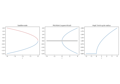
Henri Poincaré’s qualitative program (above) raised a natural next question: how does a fixed point’s classification change as a parameter varies? Aleksandr Andronov’s work on nonlinear oscillations, from 1929 to 1937, gave the question a systematic treatment. With Lev Pontryagin he introduced structural stability (“rough systems”) and studied the elementary ways a system’s qualitative behavior changes abruptly when a parameter crosses a critical value. A saddle-node bifurcation creates or destroys a pair of fixed points, a pitchfork bifurcation splits one stable state into two, and a Hopf bifurcation (named for Eberhard Hopf’s 1942 general theorem) creates a limit cycle from a spiral fixed point that loses stability.

Implementation: mathematicskit.ode_dynamics.systems.bifurcations.saddle_node_fixed_points(), pitchfork_fixed_points(), and hopf_limit_cycle_radius() give the closed-form fixed points or limit-cycle radius for each normal form, checked against numerical integration.

References: A. A. Andronov and L. Pontryagin, “Systèmes grossiers,” Doklady Akademii Nauk SSSR 14(5) (1937), 247-250.

Saddle-node, pitchfork, and Hopf bifurcation diagrams

1952 – Curtiss and Hirschfelder: Stiffness and BDF #

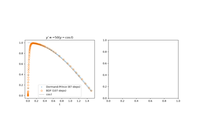
Charles Curtiss and Joseph Hirschfelder, integrating chemical-kinetics equations, found that explicit methods crawled along with tiny steps even where the solution was perfectly smooth. They called such equations stiff and illustrated the problem with

\[y' = -50\,(y - \cos t).\]

After a transient of length about \(1/50\), the solution follows the slow curve \(\approx \cos t\), but an explicit method’s step stays limited by stability to about \(1/\lambda\) for decay rate \(\lambda\). Their remedy was the backward differentiation formulas: fit a polynomial through past values and require it to satisfy the ODE at the new time point. BDF1 is backward Euler, and BDF2 is \(\tfrac32 y_{n+1} - 2y_n + \tfrac12 y_{n-1} = h f(t_{n+1}, y_{n+1})\). C. William Gear’s 1971 variable-order, variable-step BDF code (DIFSUB) made them the workhorse of stiff integration. For their original \(\lambda = 50\) the problem is only mildly stiff, and an explicit adaptive method is still competitive. By \(\lambda = 50{,}000\) Dormand-Prince needs almost 200 times as many steps as BDF.

Implementation: mathematicskit.integrators.stiff_integrate() with method="BDF" wraps scipy’s variable-order BDF (Shampine and Reichelt’s numerical differentiation formulas, orders 1-5). The tests check it against the exact solution of a stiff equation with \(\lambda = 10^4\).

References: C. F. Curtiss and J. O. Hirschfelder, “Integration of Stiff Equations,” Proceedings of the National Academy of Sciences 38 (1952), 235-243; C. W. Gear, Numerical Initial Value Problems in Ordinary Differential Equations (Prentice-Hall, 1971).

Curtiss and Hirschfelder: stiffness and BDF

1961-1962 – FitzHugh, Nagumo, and the Excitable Neuron #

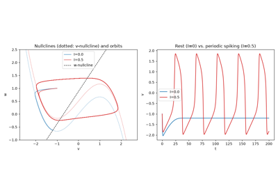
Hodgkin and Huxley’s 1952 model of the squid giant axon uses four coupled nonlinear equations. Richard FitzHugh reduced its essential behavior to two. The first is a fast voltage-like variable \(v\) with a cubic nullcline. The second is a slow recovery variable \(w\):

\[\dot v = v - \frac{v^3}{3} - w + I, \qquad \dot w = \varepsilon(v + a - bw).\]

In 1962 Jin-ichi Nagumo and colleagues built the same equations as an electronic circuit. In the phase plane, the model explains excitability: a small stimulus decays, while one past a threshold fires a full spike. When the injected current \(I\) makes the trace of the Jacobian at rest positive, the rest state gives way to repetitive firing on a relaxation limit cycle.

Implementation: mathematicskit.ode_dynamics.systems.excitable.FitzHughNagumo integrates the model. fitzhugh_nagumo_fixed_point() solves the nullcline cubic, and fitzhugh_nagumo_hopf_currents() gives the currents at which the rest state loses and regains stability, \(v_H = \pm\sqrt{1 - \varepsilon b}\). The tests check that the Jacobian’s trace vanishes at those currents.

References: R. FitzHugh, “Impulses and Physiological States in Theoretical Models of Nerve Membrane,” Biophysical Journal 1(6) (1961), 445-466; J. Nagumo, S. Arimoto, and S. Yoshizawa, “An Active Pulse Transmission Line Simulating Nerve Axon,” Proceedings of the IRE 50(10) (1962), 2061-2070.

FitzHugh-Nagumo: excitability and spiking

1963 – Lorenz and Deterministic Chaos #

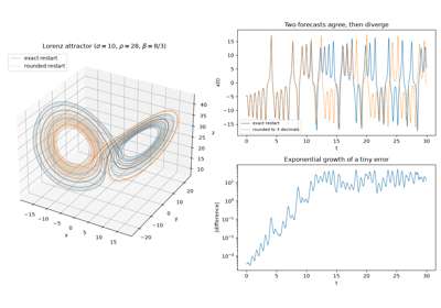
In 1961 Edward Lorenz was running a simplified 12-variable weather model on an early computer. He restarted a simulation midway, typing in values from a printout rounded to three decimal places instead of the machine’s six. Within a few simulated months the rerun had diverged completely from the original. His 1963 paper isolated the same sensitivity to initial conditions in a three-variable convection model simple enough to analyze fully. It launched the modern study of deterministic chaos, and Lorenz’s later talks gave popular science the phrase “the butterfly effect.”

Connection: the trace-determinant stability analysis used throughout this package classifies the Lorenz system’s fixed points. The bifurcation, limit-cycle, and Poincaré-section tools (above) are the general toolkit that chaos theory built to make sense of what Lorenz found.

References: E. N. Lorenz, “Deterministic Nonperiodic Flow,” Journal of the Atmospheric Sciences 20(2) (1963), 130-141.

Lorenz’s butterfly effect: deterministic chaos

Lorenz's butterfly effect: deterministic chaos

1963 – Dahlquist’s A-Stability #

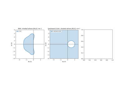
Applied to the test equation \(y' = \lambda y\), one step of a method multiplies \(y\) by a stability function \(R(z)\), with \(z = \lambda h\). Germund Dahlquist called a method A-stable if \(|R(z)| \le 1\) on the entire left half-plane \(\operatorname{Re} z \le 0\). For such a method, no decaying component can ever be amplified, whatever the step size, so the step can be chosen for accuracy alone. Explicit methods are never A-stable: their \(R\) is a polynomial, which is unbounded, and RK4 is stable on the negative real axis only down to \(z \approx -2.785\). Backward Euler, with \(R(z) = 1/(1 - z)\), is A-stable. Dahlquist’s second barrier showed that an A-stable linear multistep method has order at most 2, and that the trapezoidal rule has the smallest error constant among them. Getting past that barrier is what implicit Runge-Kutta methods do (Butcher and Ehle, below).

Implementation: mathematicskit.integrators.implicit_euler_integrate() alongside rk4_integrate(), with each method’s \(R(z)\) in stability_function() and its region drawn by mathematicskit.ode_dynamics.visualizers.plot_stability_regions(). The tests check that at \(\lambda h = 100\) backward Euler follows the exact solution while RK4 blows up, and that backward Euler’s region contains the whole sampled left half-plane.

References: G. Dahlquist, “A Special Stability Problem for Linear Multistep Methods,” BIT 3 (1963), 27-43.

Dahlquist’s A-stability: backward Euler vs RK4

Dahlquist's A-stability: backward Euler vs RK4

1964-1969 – Butcher, Ehle, and Radau IIA #

John Butcher developed the algebraic theory of Runge-Kutta methods and, in 1964, fully implicit methods whose stages sit at Gauss and Radau quadrature points. These reach order \(2s\) or \(2s - 1\) with \(s\) stages. Byron Ehle showed in 1969 that their stability functions are Padé approximants to \(e^z\), and that the Radau IIA methods are not only A-stable but L-stable: \(R(z) \to 0\) as \(z \to -\infty\), so infinitely stiff components are damped out in a single step. The trapezoidal rule, by contrast, has \(R \to -1\), so stiff components persist as step-to-step oscillations. The three-stage, order-5 Radau IIA method,

\[R(z) = \frac{1 + \tfrac25 z + \tfrac1{20} z^2} {1 - \tfrac35 z + \tfrac3{20} z^2 - \tfrac1{60} z^3},\]

is the engine of Hairer and Wanner’s RADAU5 code. It gets past Dahlquist’s order-2 barrier because it is not a multistep method. On the stiff van der Pol oscillator with \(\mu = 1000\), it needs about 1,200 steps where an explicit adaptive method needs about 1.7 million.

Implementation: mathematicskit.integrators.stiff_integrate() with method="Radau" (the default) wraps scipy’s Radau IIA implementation.

References: J. C. Butcher, “Implicit Runge-Kutta Processes,” Mathematics of Computation 18 (1964), 50-64; B. L. Ehle, “On Padé Approximations to the Exponential Function and A-Stable Methods for the Numerical Solution of Initial Value Problems,” Research Report CSRR 2010, University of Waterloo (1969); E. Hairer and G. Wanner, Solving Ordinary Differential Equations II: Stiff and Differential-Algebraic Problems (Springer, 2nd ed. 1996), sec. IV.5 and IV.8.

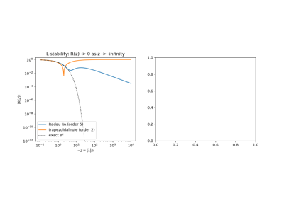
Butcher, Ehle and Radau IIA: L-stable implicit Runge-Kutta

1966 – Robertson’s Stiff Chemical Kinetics #

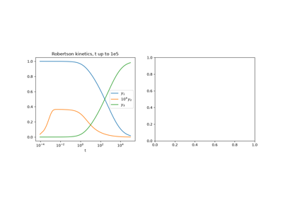
H. H. Robertson modeled an autocatalytic reaction among three species with rate constants spanning nine orders of magnitude:

\[y_1' = -0.04\,y_1 + 10^4\,y_2 y_3,\quad y_2' = 0.04\,y_1 - 10^4\,y_2 y_3 - 3\times10^7\,y_2^2,\quad y_3' = 3\times10^7\,y_2^2.\]

The intermediate \(y_2\) reaches a quasi-steady value within about \(10^{-4}\) time units, while \(y_1\) and \(y_3\) evolve over \(10^5\) units and beyond. Total mass \(y_1 + y_2 + y_3 = 1\) is conserved. Robertson’s system became the standard benchmark for stiff solvers, and it shows the problem vividly: to reach \(t = 40\), explicit Dormand-Prince needs about 35,000 steps, while an implicit method needs under 100.

Implementation: mathematicskit.integrators.stiff_integrate() (Radau IIA by default) integrates the system to \(t = 10^5\) in fewer than 200 steps, conserving mass to rounding error.

References: H. H. Robertson, “The Solution of a Set of Reaction Rate Equations,” in J. Walsh (ed.), Numerical Analysis: An Introduction (Academic Press, 1966), 178-182.

Robertson’s stiff chemical kinetics

Robertson's stiff chemical kinetics

1968 – Prigogine, Lefever, and the Brusselator #

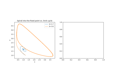
Chemists long doubted that a homogeneous chemical reaction could oscillate. It seemed to conflict with the approach to equilibrium that thermodynamics requires. Ilya Prigogine and René Lefever showed that a system held far from equilibrium can oscillate. Their minimal reaction scheme, later nicknamed the “Brusselator,” has rate equations

\[\dot x = a - (b + 1)x + x^2 y, \qquad \dot y = bx - x^2 y.\]

The single fixed point \((a, b/a)\) has a Jacobian with determinant \(a^2\) and trace \(b - 1 - a^2\). It therefore loses stability in a Hopf bifurcation at exactly \(b_c = 1 + a^2\), beyond which the concentrations oscillate on a limit cycle. The model became a standard example for the theory of dissipative structures, which contributed to Prigogine’s 1977 Nobel Prize in Chemistry. The Belousov-Zhabotinsky reaction then gave laboratory chemists a real oscillating reaction to study.

Implementation: mathematicskit.ode_dynamics.systems.chemical_oscillators.Brusselator integrates the model, and brusselator_hopf_threshold() returns \(b_c\). The tests check that the numerical Jacobian’s trace vanishes there, and that oscillations appear only above it.

References: I. Prigogine and R. Lefever, “Symmetry Breaking Instabilities in Dissipative Systems. II,” Journal of Chemical Physics 48(4) (1968), 1695-1700.

The Brusselator’s Hopf bifurcation

The Brusselator's Hopf bifurcation

1973 – De Boor and Swartz: Collocation for Boundary-Value Problems #

A two-point boundary-value problem fixes conditions at both ends, as in \(y'' = f(x, y, y')\) with \(y(a) = \alpha\) and \(y(b) = \beta\), so there is no initial state to march forward from. Shooting guesses the missing initial slope and corrects it, but it inherits any instability of the initial-value problem. Collocation instead solves for the whole solution at once: a piecewise polynomial on a mesh is required to satisfy the ODE exactly at \(k\) collocation points per interval and to meet the boundary conditions, which gives one nonlinear system for Newton’s method. Carl de Boor and Blair Swartz proved that with Gauss points the error at the mesh nodes is \(O(h^{2k})\), far better than the \(O(h^k)\) of the polynomial pieces themselves (“superconvergence”). That theory underlies Ascher, Christiansen, and Russell’s COLSYS (1979) and Kierzenka and Shampine’s residual-controlled solver behind scipy.integrate.solve_bvp(), which uses the related three-point Lobatto IIIA scheme. Because the problem is solved globally, a nonlinear BVP can have several solutions. Bratu’s problem \(y'' + \lambda e^y = 0\), \(y(0) = y(1) = 0\) has two for \(\lambda < 3.51\), and the initial guess decides which one Newton finds.

Implementation: mathematicskit.integrators.collocation_bvp() wraps scipy.integrate.solve_bvp() in the integrators’ rhs(state, x, params) convention and returns a BVPResult. The tests recover \(\sin x\) and both of Bratu’s closed-form solutions.

References: C. de Boor and B. Swartz, “Collocation at Gaussian Points,” SIAM Journal on Numerical Analysis 10 (1973), 582-606; J. Kierzenka and L. F. Shampine, “A BVP Solver Based on Residual Control and the MATLAB PSE,” ACM Transactions on Mathematical Software 27 (2001), 299-316; G. Bratu, “Sur les équations intégrales non linéaires,” Bulletin de la Société Mathématique de France 42 (1914), 113-142.

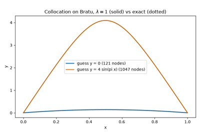
De Boor and Swartz: collocation for boundary-value problems

1975 – Kuramoto’s Synchronization Transition #

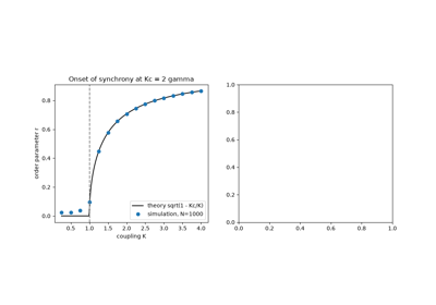
Fireflies flash in unison, heart pacemaker cells fire together, and applause can fall into a common rhythm. Arthur Winfree had modeled such collective synchrony in 1967. Yoshiki Kuramoto found a version simple enough to solve exactly: \(N\) oscillators, each with its own natural frequency \(\omega_i\), all pulling on one another’s phases:

\[\dot\theta_i = \omega_i + \frac{K}{N}\sum_{j=1}^N \sin(\theta_j - \theta_i), \qquad r e^{i\psi} = \frac1N\sum_j e^{i\theta_j}.\]

The order parameter \(r\) measures coherence. For weak coupling it stays near zero. At a critical coupling \(K_c = 2/(\pi g(0))\), where \(g\) is the distribution of natural frequencies, a synchronized cluster forms spontaneously, a phase transition in time rather than in space. For a Lorentzian \(g\) of half-width \(\gamma\), Kuramoto obtained \(r = \sqrt{1 - 2\gamma/K}\) exactly.

Implementation: mathematicskit.ode_dynamics.systems.synchronization.KuramotoModel integrates the model in \(O(N)\) mean-field form, passing the natural frequencies through the integrator’s params array. kuramoto_order_parameter() and kuramoto_lorentzian_order_parameter() give the simulated and theoretical coherence. With \(N = 1000\) oscillators, the tests match the theory to within 0.03.

References: Y. Kuramoto, “Self-entrainment of a population of coupled non-linear oscillators,” in International Symposium on Mathematical Problems in Theoretical Physics, Lecture Notes in Physics 39 (Springer, 1975), 420-422; S. H. Strogatz, “From Kuramoto to Crawford: exploring the onset of synchronization in populations of coupled oscillators,” Physica D 143 (2000), 1-20.

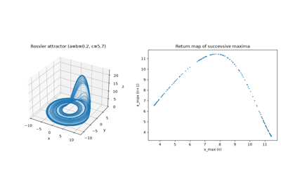
The Kuramoto synchronization transition

1976 – Rössler’s Minimal Chaotic Flow #

Otto Rössler looked for a chaotic flow even simpler than Lorenz’s, one whose mechanism could be seen directly. He built it around a geometric picture of how chaos arises: stretch, then fold, like kneading dough. His system has a single nonlinear term:

\[\dot x = -y - z, \qquad \dot y = x + ay, \qquad \dot z = b + z(x - c).\]

Orbits spiral outward in the \((x, y)\) plane until \(x\) passes \(c\). Then \(z\) spikes, lifting the orbit and folding it back toward the center. For \(a = b = 0.2\), \(c = 5.7\), the result is a chaotic attractor. Plotting each loop’s maximum of \(x\) against the previous one gives a thin, single-humped curve, which connects the continuous flow to the one-dimensional maps behind Feigenbaum’s universality (below).

Implementation: mathematicskit.ode_dynamics.systems.chaotic_flows.RosslerSystem integrates the flow, and rossler_fixed_points() gives its two fixed points in closed form, as the roots of \(ay^2 + cy + b = 0\). The tests check the fixed points, that the attractor stays bounded, and that nearby trajectories separate.

References: O. E. Rössler, “An Equation for Continuous Chaos,” Physics Letters A 57(5) (1976), 397-398.

The Rossler attractor

1978 – Feigenbaum’s Universality #

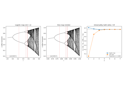
Mitchell Feigenbaum studied the logistic map’s period-doubling route to chaos numerically, on a programmable calculator. He noticed that the parameter intervals between successive period doublings shrink by a constant ratio. The same ratio, \(\delta \approx 4.6692\), governs the period-doubling cascade of a huge class of unrelated one-dimensional maps with a single smooth maximum. It was one of the first, and remains one of the most striking, universal quantitative laws of the transition to chaos, holding across very different physical systems.

Implementation: mathematicskit.ode_dynamics.systems.logistic_map.LogisticMap and bifurcation_diagram() reproduce the cascade; estimate_feigenbaum_delta() estimates \(\delta\) from the first few numerically located bifurcation points.

References: M. J. Feigenbaum, “Quantitative Universality for a Class of Nonlinear Transformations,” Journal of Statistical Physics 19(1) (1978), 25-52.

Feigenbaum’s universal constant in the period-doubling cascade

Feigenbaum's universal constant in the period-doubling cascade

1980 – Dormand and Prince: Embedded Pairs and Adaptive Steps #

A fixed step wastes effort where the solution is smooth and loses accuracy where it changes quickly. Erwin Fehlberg (1969) showed how an embedded pair, two Runge-Kutta formulas of orders \(p\) and \(p - 1\) sharing the same stages, estimates the local error almost for free, and a controller then adjusts \(h\) to keep that estimate below a tolerance. John Dormand and Peter Prince tuned a 5(4) pair so that the fifth-order solution, the one actually kept, has a very small error constant. Its last stage is also the first stage of the next step (“first same as last”). 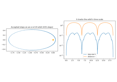Their pair became the default in MATLAB’s ode45 and scipy’s RK45. On an eccentric Kepler orbit the step shrinks sharply at every close approach and grows again far from the Sun.

Implementation: mathematicskit.integrators.dopri5_integrate() (Numba-compiled, with the same atol + rtol * |y| error norm as scipy). The tests check it against the harmonic oscillator’s exact solution, that tighter tolerances take more steps, and that it agrees with fine-step RK4.

References: J. R. Dormand and P. J. Prince, “A Family of Embedded Runge-Kutta Formulae,” Journal of Computational and Applied Mathematics 6 (1980), 19-26; E. Fehlberg, “Low-Order Classical Runge-Kutta Formulas with Stepsize Control and Their Application to Some Heat Transfer Problems,” NASA Technical Report R-315 (1969).

Dormand-Prince: embedded pairs and adaptive step size

1990 – Yoshida’s Symplectic Composition #

Haruo Yoshida showed how to raise the order of a symmetric integrator while keeping it symplectic, by composing it with itself. Three leapfrog substeps of lengths \(w_1 h, w_0 h, w_1 h\), with

\[w_1 = \frac{1}{2 - 2^{1/3}},\qquad w_0 = -\frac{2^{1/3}}{2 - 2^{1/3}},\]

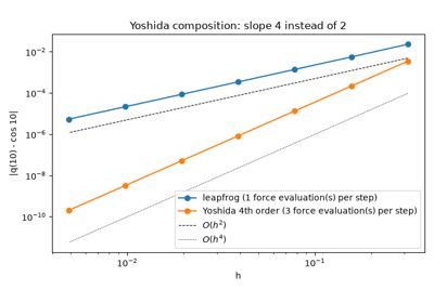
cancel the leading \(h^3\) error term and give a fourth-order symplectic method. The middle substep runs backwards in time. Repeating the construction reaches orders 6, 8, and beyond. Because every substep is symplectic, the composition keeps leapfrog’s bounded long-time energy error while converging far faster, which made it popular in celestial mechanics and accelerator physics.

Implementation: mathematicskit.integrators.yoshida4_integrate(). The tests check that halving \(h\) divides the error by about 16.

References: H. Yoshida, “Construction of Higher Order Symplectic Integrators,” Physics Letters A 150 (1990), 262-268.

Yoshida’s symplectic composition: fourth order from leapfrog

Yoshida's symplectic composition: fourth order from leapfrog