Breakthroughs in Geophysics#
Geophysics began with two forces that act at a distance: the pull of the
Earth’s mass and the turn of a compass needle. Gilbert made the Earth a magnet
and Newton made it a rotating, flattened fluid. The 18th century measured that
shape with pendulums and plumb lines, and Cavendish weighed the planet. Gauss
and Stokes turned magnetic and gravity measurements into fields with an exact
mathematical form. In the 20th century rocks showed that the field had reversed
many times, satellites remeasured the shape of the Earth and then weighed its
moving water month by month. This chronology traces the results behind
earthsciencekit.geophysics. Every example uses deterministic synthetic
inputs; none inverts real observations.
1600 – Gilbert’s Magnetic Earth#
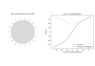
William Gilbert carved a sphere of lodestone, his terrella, and carried a
small dip needle over it. The needle lay flat at the terrella’s equator, stood
vertical at its poles and dipped in between, as compass needles did at sea.
Gilbert concluded that the Earth itself is a great magnet. For an axial dipole
the inclination obeys tan(I) = 2 tan(latitude), and the field at the poles
is twice that at the equator.
Implementation: dipole_field() and
dipole_inclination() (new). The example
draws dip needles around a terrella and checks the factor of two.
References: W. Gilbert, De Magnete, Magneticisque Corporibus, et de Magno Magnete Tellure (London: Peter Short, 1600).
1687 – Newton’s Oblate Earth#
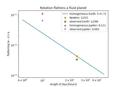
Isaac Newton argued that a rotating fluid Earth must bulge at the equator.
Treating it as homogeneous, he balanced the weight of water in two canals
reaching the centre, one from the pole and one from the equator, and found the
axes in the ratio 229 to 230, a flattening of 1/230. The modern value, 1/298,
is smaller because the Earth’s mass is concentrated toward its centre. For a
slowly rotating homogeneous fluid the flattening is 5 m / 4, where m is
the ratio of centrifugal to gravitational acceleration at the equator.
Implementation: centrifugal_ratio() and
homogeneous_flattening() (new). The example
recovers Newton’s 1/230 and compares the Earth with Jupiter.
References: I. Newton, Philosophiæ Naturalis Principia Mathematica (London, 1687), Book III, Propositions 18-20.
1743 – Clairaut’s Theorem#
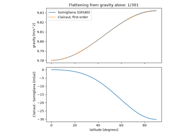
Alexis Clairaut showed that a rotating Earth in hydrostatic equilibrium, made
of layers of any density, has a gravity that grows from equator to pole by the
fraction 5 m / 2 - f. Pendulum measurements of gravity at a few latitudes
therefore give the flattening without measuring any arc of meridian. The
first-order formula matches the exact normal gravity of today’s reference
ellipsoid, given by Somigliana’s closed form, to 50 parts per million.
Implementation: clairaut_gravity() and
normal_gravity() (new). The example
recovers a flattening of 1/301 from equatorial and polar gravity alone.
References: A.-C. Clairaut, Théorie de la figure de la Terre, tirée des principes de l’hydrostatique (Paris: David fils, 1743). H. Moritz, “Geodetic Reference System 1980,” Bulletin Géodésique 54 (1980): 395-405.
1749 – Bouguer’s Mountain Attraction#
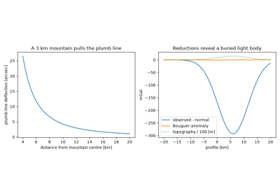
On the French geodetic expedition to Peru, Pierre Bouguer tried to measure how far the volcano Chimborazo pulled a plumb line aside. The deflection he found was much smaller than he expected, but the attempt was the first to detect a mountain’s gravity. At Quito he also found gravity on the high plateau larger than the height alone predicted, because the rock under the station attracts too. Removing that slab (the Bouguer correction) and the effect of height (the free-air correction) leaves the Bouguer anomaly of buried masses that gravity surveys still map.
Implementation: sphere_gravity(),
bouguer_correction(),
free_air_correction() and
bouguer_anomaly() (new). The example
computes the plumb-line deflection beside a model mountain and recovers a
buried body from gravity observed on topography.
References: P. Bouguer, La figure de la Terre, déterminée par les observations de Messieurs Bouguer et de La Condamine (Paris: Jombert, 1749).
1798 – Cavendish Weighs the Earth#
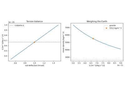
Henry Cavendish hung a 1.8 m rod carrying two small lead balls from a fine wire and brought two 158 kg balls close to them. The rod twisted by about a milliradian, and the period of its free swing calibrated the wire. The experiment gives the gravitational constant, and with surface gravity the mean density of the Earth: Cavendish found 5.48 times that of water, about twice the density of surface rocks, so the interior must be much denser.
Implementation:
torsion_balance_gravitational_constant() and
earth_mean_density() (new).
References: H. Cavendish, “Experiments to determine the density of the Earth,” Philosophical Transactions of the Royal Society of London 88 (1798): 469-526.
1839 – Gauss’s Spherical-Harmonic Geomagnetic Field#
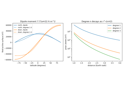
Carl Friedrich Gauss wrote the magnetic potential as a series of spherical
harmonics and fitted its coefficients to observations from around the world.
The fit showed that the field comes almost entirely from inside the Earth, and
its degree-1 coefficients gave the moment and tilt of the best-fitting dipole.
The same expansion is still the International Geomagnetic Reference Field.
Each degree n falls off as r**-(n + 2), so the dipole dominates far from
the core.
Implementation: zonal_field() and
gauss_dipole_moment() (new). The example
finds a moment of 7.7e22 A m^2 and a tilt of 9.4 degrees from the IGRF-13
coefficients for 2020.
References: C. F. Gauss, “Allgemeine Theorie des Erdmagnetismus,” in Resultate aus den Beobachtungen des magnetischen Vereins im Jahre 1838 (Leipzig, 1839): 1-57. P. Alken et al., “International Geomagnetic Reference Field: the thirteenth generation,” Earth, Planets and Space 73 (2021): 49.
Gauss’s spherical-harmonic geomagnetic field (1839)
1849 – Stokes’s Geoid Formula#
George Gabriel Stokes showed that gravity measured over the whole surface
fixes the shape of the level surface, the geoid, without any assumption about
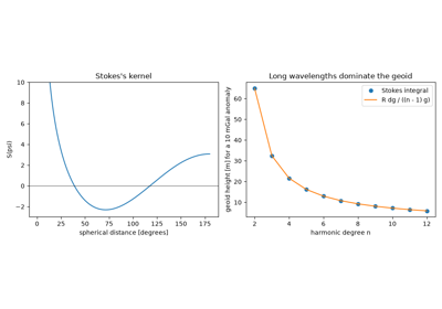
the density inside. The geoid height at a point is the integral of the gravity
anomaly over the globe, weighted by a kernel of spherical distance alone. An
anomaly of spherical-harmonic degree n gives a geoid of the same shape
scaled by R / ((n - 1) g), so the geoid is dominated by long wavelengths.
Implementation: stokes_function() and
degree_geoid_height() (new). The example
integrates the kernel numerically against zonal anomalies and checks the
1 / (n - 1) law.
References: G. G. Stokes, “On the variation of gravity at the surface of the Earth,” Transactions of the Cambridge Philosophical Society 8 (1849): 672-695.
1906 – Brunhes’s Reversed Magnetization#
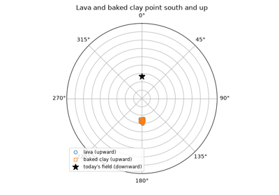
Bernard Brunhes, with Pierre David, studied a lava flow at Pontfarein in the Massif Central and the clay it had baked as it flowed. Both were magnetized in the same direction, nearly opposite to today’s field. The clay could only have acquired its magnetization from the field as it cooled, so the field itself had pointed the other way. At the site’s latitude of 45 degrees a reversed dipole gives a declination of 180 degrees and an inclination of -63 degrees.
Implementation: field_elements() (new).
The example plots lava and baked-clay directions against today’s field.
References: B. Brunhes, “Recherches sur la direction d’aimantation des roches volcaniques,” Journal de Physique Théorique et Appliquée 5 (1906): 705-724.
1909 – Love Numbers#
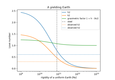
Kelvin had argued from the ocean tides that the Earth is about as rigid as
steel. Augustus Love described the Earth’s yielding to the tidal potential by
two numbers: h, the body-tide uplift as a fraction of the equilibrium tide,
and k, the extra potential of the deformed Earth as a fraction of the tidal
potential. A uniform elastic sphere as rigid as steel has k2 near 0.47; the
real Earth, with its fluid core, has h2 = 0.61 and k2 = 0.30.
Gravimeters see the tide amplified by 1 + h - 3 k / 2, about 1.16.
Implementation: love_number_h2(),
love_number_k2() and
tidal_gravimetric_factor() (new), for
Kelvin’s uniform incompressible sphere.
References: A. E. H. Love, “The yielding of the Earth to disturbing forces,” Proceedings of the Royal Society of London A 82 (1909): 73-88. W. Thomson, “On the rigidity of the Earth,” Philosophical Transactions of the Royal Society of London 153 (1863): 573-582.
1919 – Larmor’s Self-Exciting Dynamo#
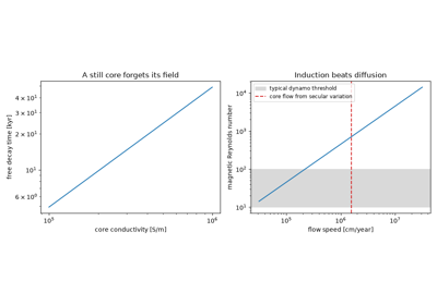
Joseph Larmor asked how a body such as the Sun could become a magnet, and proposed that conducting fluid moving through a magnetic field could induce the currents that keep the field alive, like a self-exciting dynamo. The Earth needs one: a field left in a still iron core would decay in tens of thousands of years, yet rocks record a field for more than three billion years. Core flow of a fraction of a millimetre per second gives a magnetic Reynolds number in the hundreds, enough for induction to beat diffusion.
Implementation: magnetic_decay_time() and
magnetic_reynolds_number() (new).
References: J. Larmor, “How could a rotating body such as the Sun become a magnet?” Report of the British Association for the Advancement of Science (1919): 159-160. W. M. Elsasser, “Induction effects in terrestrial magnetism. Part I. Theory,” Physical Review 69 (1946): 106-116.
1929 – Matuyama’s Reversed Epoch#
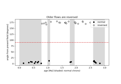
Motonori Matuyama measured the magnetization of basalts from Japan, Korea and Manchuria. The youngest flows were magnetized along today’s field, but older, early Quaternary flows pointed the opposite way. He concluded that the field had been reversed for a long interval before the present one, now called the Matuyama chron. A flow is reversed when its direction lies more than 90 degrees from the present axial dipole field at the site.
Implementation: direction_angle() (new).
The example classifies a synthetic sequence of dated flows by that angle.
References: M. Matuyama, “On the direction of magnetisation of basalt in Japan, Tyôsen and Manchuria,” Proceedings of the Imperial Academy 5 (1929): 203-205.
1956 – Runcorn’s Apparent Polar Wander#
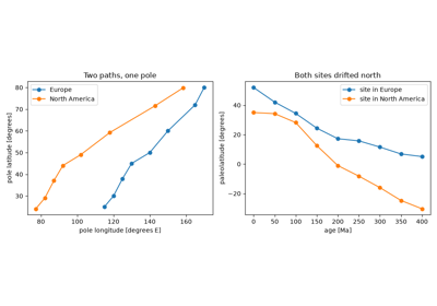
Keith Runcorn and his colleagues converted the magnetization directions of old rocks into virtual geomagnetic poles. British rocks gave poles that wandered farther from the present pole with age. When Runcorn added North American rocks, their path ran parallel to the European one but about 30 degrees to the west. One dipole cannot have two poles, so the continents had moved apart: closing the Atlantic brings the two paths together. Runcorn became one of the first geophysicists to accept continental drift.
Implementation: virtual_geomagnetic_pole()
and paleolatitude() (new). The example
builds synthetic paths related by the Bullard et al. (1965) fit of the Atlantic
and recovers them from site directions.
References: S. K. Runcorn, “Paleomagnetic comparisons between Europe and North America,” Proceedings of the Geological Association of Canada 8 (1956): 77-85. E. Bullard, J. E. Everett and A. G. Smith, “The fit of the continents around the Atlantic,” Philosophical Transactions of the Royal Society of London A 258 (1965): 41-51.
1958 – Rikitake’s Two-Disc Dynamo#
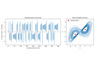
Tsuneji Rikitake coupled two disc dynamos, each driven by the same torque and each feeding the coil of the other. The currents never settle: they oscillate about one of two steady states of opposite sign and at irregular intervals jump to the other. The model showed that a deterministic dynamo can reverse its field without any outside trigger, with polarity intervals of very unequal length, as in the geological record.
Implementation: simulate_rikitake_dynamo()
and rikitake_fixed_point() (new).
References: T. Rikitake, “Oscillations of a system of disk dynamos,” Proceedings of the Cambridge Philosophical Society 54 (1958): 89-105.
1958 – King-Hele’s Flattening from Satellite Orbits#
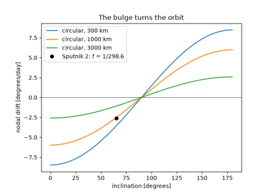
The equatorial bulge torques an inclined orbit and makes its node drift westward at a rate proportional to J2. Robert Merson and Desmond King-Hele timed the drift of Sputnik 2 and found a flattening of 1/298.3, not the 1/297 of the International Ellipsoid that surveyors had used since 1924. A few months of tracking one satellite had improved on two centuries of arc measurement.
Implementation: nodal_precession_rate() and
flattening_from_j2() (new). The example
recovers J2 from Sputnik 2’s nodal drift of about -2.6 degrees per day.
References: R. H. Merson and D. G. King-Hele, “A new value for the Earth’s flattening, derived from measurements of satellite orbits,” Nature 182 (1958): 640-641.
King-Hele’s flattening from satellite orbits (1958)
1964 – Cox, Doell and Dalrymple’s Polarity Timescale#
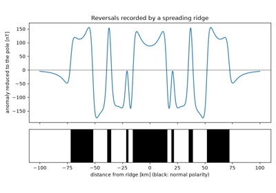
Allan Cox, Richard Doell and Brent Dalrymple dated lava flows from around the world by potassium-argon and measured their polarity. Flows of the same age had the same polarity everywhere, so reversals are global and can be put on a clock: the normal Brunhes epoch, the reversed Matuyama with short normal events, and the normal Gauss. The timescale turned the magnetic stripes at ridges into a speedometer for seafloor spreading.
Implementation: block_magnetic_anomaly()
(new). The example builds the anomaly profile across a ridge from a modern
version of the timescale, including the Jaramillo event found in 1966.
References: A. Cox, R. R. Doell and G. B. Dalrymple, “Reversals of the Earth’s magnetic field,” Science 144 (1964): 1537-1543. J. G. Ogg, “Geomagnetic polarity time scale,” in F. M. Gradstein et al. (eds.), Geologic Time Scale 2020 (Amsterdam: Elsevier, 2020).
Cox, Doell and Dalrymple’s polarity timescale (1964)
2002 – GRACE Gravity Changes#
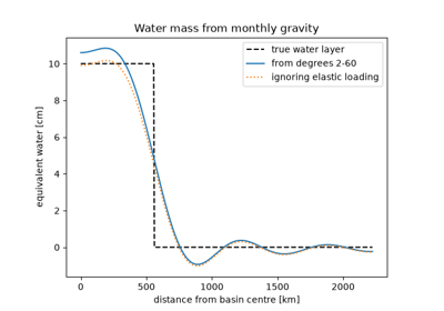
The twin GRACE satellites, launched in March 2002, measured the distance between them to microns. Its changes gave a new global gravity field every month, and the differences between months show where water, ice and groundwater moved. Each change of a Stokes coefficient becomes a layer of equivalent water, after allowing for the elastic Earth sinking under the load.
Implementation: equivalent_water_height()
(new). The example recovers a basin’s seasonal water from coefficients up to
degree 60 and shows how ignoring elastic loading underestimates it.
References: J. Wahr, M. Molenaar and F. Bryan, “Time variability of the Earth’s gravity field: Hydrological and oceanic effects and their possible detection using GRACE,” Journal of Geophysical Research 103 (1998): 30205-30229. B. D. Tapley, S. Bettadpur, J. C. Ries, P. F. Thompson and M. M. Watkins, “GRACE measurements of mass variability in the Earth system,” Science 305 (2004): 503-505.
See also#
Geophysics: units, equations and validation for conventions, equations and checks.
Breakthroughs in Plate Tectonics, whose magnetic stripes and isostasy rest on these results.