Love numbers (1909)

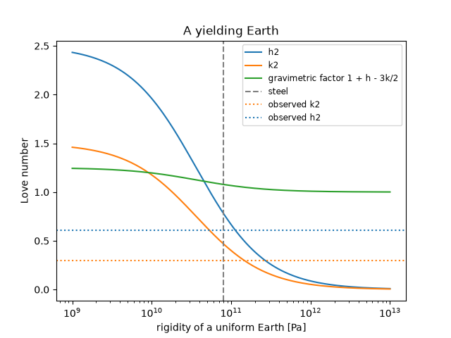
Kelvin had argued from the ocean tides that the Earth is about as rigid as steel. Augustus Love described the Earth’s yielding to the tidal potential by two numbers: h, the ratio of the body-tide uplift to the equilibrium tide, and k, the extra potential of the deformed Earth. A uniform elastic sphere as rigid as steel has k2 near 0.47; the real Earth, with a fluid core, has h2 = 0.61 and k2 = 0.30. Gravimeters see the tide amplified by 1 + h - 3 k / 2, about 1.16.

import matplotlib.pyplot as plt
import numpy as np

from earthsciencekit.geophysics import love_number_h2, love_number_k2, tidal_gravimetric_factor

density, gravity, radius = 5514.0, 9.82, 6.371e6
rigidity = np.logspace(9, 13, 200)
h2, k2 = love_number_h2(rigidity, density, gravity, radius), love_number_k2(rigidity, density, gravity, radius)
steel = 8e10
steel_k2 = love_number_k2(steel, density, gravity, radius)
assert 0.3 < steel_k2 < 0.6
assert np.isclose(tidal_gravimetric_factor(0.61, 0.30), 1.16)
effective = rigidity[np.argmin(np.abs(k2 - 0.30))]
assert effective > steel

fig, ax = plt.subplots()
ax.semilogx(rigidity, h2, label="h2")
ax.semilogx(rigidity, k2, label="k2")
ax.semilogx(rigidity, tidal_gravimetric_factor(h2, k2), label="gravimetric factor 1 + h - 3k/2")
ax.axvline(steel, color="0.5", ls="--", label="steel")
ax.axhline(0.30, color="C1", ls=":", label="observed k2")
ax.axhline(0.61, color="C0", ls=":", label="observed h2")
ax.set(xlabel="rigidity of a uniform Earth [Pa]", ylabel="Love number", title="A yielding Earth")
ax.legend(fontsize="small")

plt.show()