Cooper and Jacob’s straight-line method (1946)

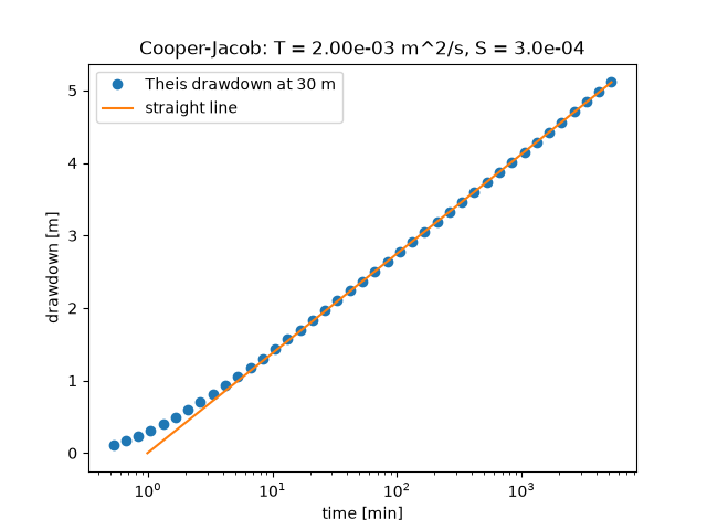
Hilton Cooper and Charles Jacob noticed that once u is small the Theis well function is just -0.5772 - ln u, so late drawdowns fall on a straight line against the logarithm of time. The drawdown gained per tenfold increase in time gives the transmissivity, and the time at which the line crosses zero drawdown gives the storativity, without matching a type curve. The example recovers both from a synthetic pumping test.

import matplotlib.pyplot as plt
import numpy as np

from earthsciencekit.hydrology import cooper_jacob_drawdown, cooper_jacob_transmissivity, theis_drawdown

rate, transmissivity, storativity, radius = 0.015, 2e-3, 3e-4, 30.0
time = np.logspace(1.5, 5.5, 41)
observed = theis_drawdown(rate, transmissivity, storativity, radius, time)
late = radius**2 * storativity / (4 * transmissivity * time) < 0.01
slope, intercept = np.polyfit(np.log10(time[late]), observed[late], 1)
fitted_transmissivity = cooper_jacob_transmissivity(rate, slope)
zero_time = 10 ** (-intercept / slope)
fitted_storativity = 2.25 * fitted_transmissivity * zero_time / radius**2
assert np.isclose(fitted_transmissivity, transmissivity, rtol=0.01) and np.isclose(fitted_storativity, storativity, rtol=0.03)

fig, ax = plt.subplots()
ax.semilogx(time / 60, observed, "o", label="Theis drawdown at 30 m")
line_time = np.logspace(np.log10(zero_time), 5.5, 50)
ax.semilogx(
    line_time / 60, cooper_jacob_drawdown(rate, fitted_transmissivity, fitted_storativity, radius, line_time), label="straight line"
)
ax.set(xlabel="time [min]", ylabel="drawdown [m]")
ax.set_title(f"Cooper-Jacob: T = {fitted_transmissivity:.2e} m^2/s, S = {fitted_storativity:.1e}")
ax.legend()

plt.show()