Knopoff’s Q (1964)

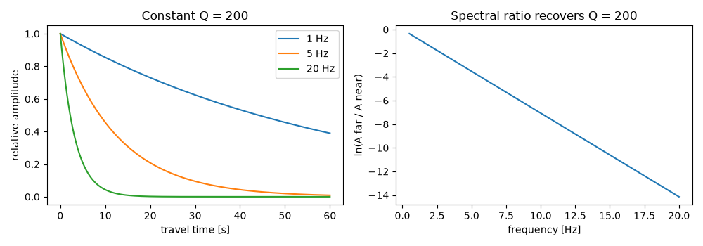
Leon Knopoff reviewed the evidence that rocks dissipate a nearly constant fraction of wave energy per cycle, whatever the frequency. With a constant quality factor Q, amplitude decays as exp(-pi f t / Q), so high frequencies die first. The log ratio of two spectra is then a straight line in frequency whose slope gives Q, the spectral-ratio method.

import matplotlib.pyplot as plt
import numpy as np

from earthsciencekit.seismology import attenuated_amplitude

Q = 200.0
frequency = np.linspace(0.5, 20, 100)
near, far = 5.0, 50.0
log_ratio = np.log(attenuated_amplitude(1, frequency, far, Q) / attenuated_amplitude(1, frequency, near, Q))
slope = np.polyfit(frequency, log_ratio, 1)[0]
Q_hat = -np.pi * (far - near) / slope
assert np.isclose(Q_hat, Q)

travel = np.linspace(0, 60, 200)
fig, axes = plt.subplots(1, 2, figsize=(10, 3.5))
for f in [1, 5, 20]:
    axes[0].plot(travel, attenuated_amplitude(1, f, travel, Q), label=f"{f} Hz")
axes[0].set(xlabel="travel time [s]", ylabel="relative amplitude", title=f"Constant Q = {Q:.0f}")
axes[0].legend()
axes[1].plot(frequency, log_ratio)
axes[1].set(xlabel="frequency [Hz]", ylabel="ln(A far / A near)", title=f"Spectral ratio recovers Q = {Q_hat:.0f}")
fig.tight_layout()

plt.show()