Horton’s infiltration capacity (1933)

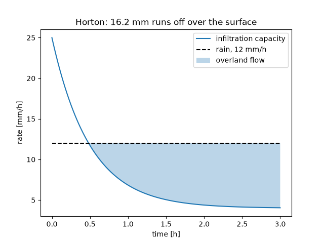
Robert Horton described the soil surface as a separator: rain up to the infiltration capacity enters the soil and feeds groundwater, and rain beyond it runs off over the surface. The capacity falls exponentially during a storm from an initial to a steady value. Overland flow produced this way, Hortonian or infiltration-excess runoff, is the shaded area where the rain exceeds the capacity.

import matplotlib.pyplot as plt
import numpy as np

from earthsciencekit.hydrology import horton_cumulative_infiltration, horton_infiltration_rate

time = np.linspace(0, 3 * 3600, 361)
capacity = horton_infiltration_rate(time, 25 / 3.6e6, 4 / 3.6e6, 1 / 1800)  # mm/h converted to m/s
rain = np.full_like(time, 12 / 3.6e6)
infiltration = np.minimum(rain, capacity)
runoff_depth = np.trapezoid(rain - infiltration, time)
total = horton_cumulative_infiltration(time[-1], 25 / 3.6e6, 4 / 3.6e6, 1 / 1800)
assert np.isclose(total, np.trapezoid(capacity, time), rtol=1e-4) and runoff_depth > 0

fig, ax = plt.subplots()
ax.plot(time / 3600, capacity * 3.6e6, label="infiltration capacity")
ax.plot(time / 3600, rain * 3.6e6, "k--", label="rain, 12 mm/h")
ax.fill_between(time / 3600, capacity * 3.6e6, rain * 3.6e6, where=rain > capacity, alpha=0.3, label="overland flow")
ax.set(xlabel="time [h]", ylabel="rate [mm/h]", title=f"Horton: {runoff_depth * 1e3:.1f} mm runs off over the surface")
ax.legend()

plt.show()