Parsons and Sclater’s depth-age law (1977)

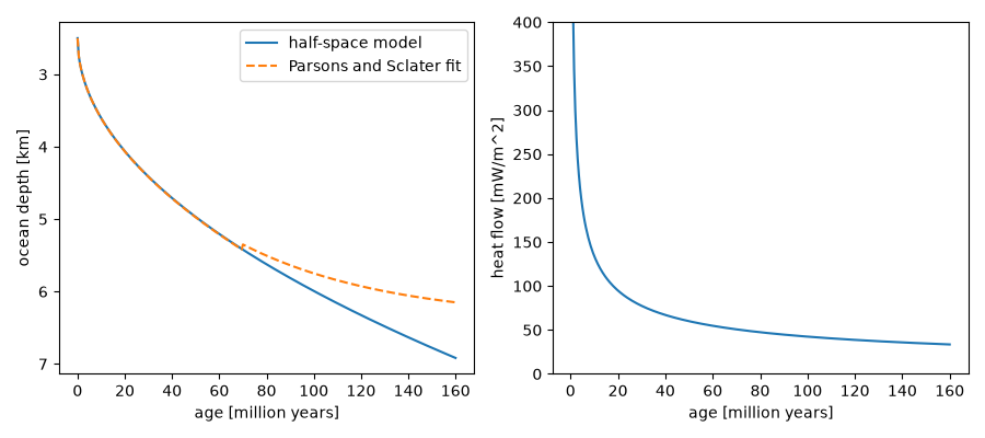
Barry Parsons and John Sclater fitted ocean depth and heat flow against sea-floor age. Out to about 70 million years the depth grows as 2500 + 350 sqrt(t) metres (t in million years), which the cooling half-space reproduces; older floor flattens, as their cooling-plate fit shows. Surface heat flow falls as one over the square root of age.

import matplotlib.pyplot as plt
import numpy as np

from earthsciencekit.plate_tectonics import halfspace_heat_flux, ocean_depth
from earthsciencekit.units import convert

age_myr = np.linspace(0, 160, 321)
age = convert(age_myr * 1e6, "year", "s")
depth = ocean_depth(age, 2500, 3300, 1000, 3e-5, 1e-6, 273, 1553)
empirical = np.where(age_myr < 70, 2500 + 350 * np.sqrt(age_myr), 6400 - 3200 * np.exp(-age_myr / 62.8))
young = age_myr < 70
np.testing.assert_allclose(depth[young], empirical[young], rtol=0.01)
flux = halfspace_heat_flux(age[1:], 1e-6, 3.3, 273, 1553)
np.testing.assert_allclose(flux * np.sqrt(age_myr[1:]), flux[0] * np.sqrt(age_myr[1]))

fig, (left, right) = plt.subplots(1, 2, figsize=(9, 4))
left.plot(age_myr, depth / 1e3, label="half-space model")
left.plot(age_myr, empirical / 1e3, "--", label="Parsons and Sclater fit")
left.invert_yaxis()
left.set(xlabel="age [million years]", ylabel="ocean depth [km]")
left.legend()
right.plot(age_myr[1:], flux * 1e3)
right.set(xlabel="age [million years]", ylabel="heat flow [mW/m^2]", ylim=(0, 400))
fig.tight_layout()

plt.show()