The Charney report’s sensitivity range (1979)

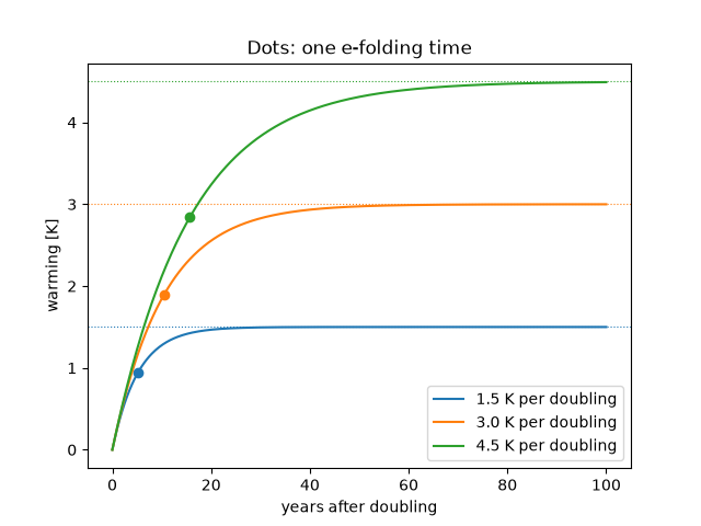
A panel of the US National Academy of Sciences chaired by Jule Charney reviewed the climate models of the day. It concluded that doubling CO2 would warm the Earth by 3 K, probably between 1.5 and 4.5 K. It also warned that ocean heat capacity would delay the warming by decades. In a one-box model the delay is the time scale C / lambda, so a more sensitive climate (a smaller lambda) also responds more slowly.

import matplotlib.pyplot as plt
import numpy as np

from earthsciencekit.climate import co2_forcing, equilibrium_warming, heat_capacity_column, response_timescale, step_temperature
from earthsciencekit.units import convert

doubling = co2_forcing(560, 280, 5.35)
capacity = heat_capacity_column(1025, 3990, 100)
years = np.linspace(0, 100, 401)
time = convert(years, "year", "s")
fig, ax = plt.subplots()
for sensitivity in [1.5, 3.0, 4.5]:
    restoring = doubling / sensitivity
    timescale = response_timescale(capacity, restoring)
    assert np.isclose(equilibrium_warming(doubling, restoring), sensitivity)
    assert np.isclose(step_temperature(doubling, restoring, capacity, timescale), sensitivity * (1 - np.exp(-1)))
    line = ax.plot(years, step_temperature(doubling, restoring, capacity, time), label=f"{sensitivity} K per doubling")[0]
    ax.axhline(sensitivity, color=line.get_color(), ls=":", lw=0.8)
    ax.plot(convert(timescale, "s", "year"), sensitivity * (1 - np.exp(-1)), "o", color=line.get_color())
ax.set(xlabel="years after doubling", ylabel="warming [K]", title="Dots: one e-folding time")
ax.legend()

plt.show()